Vegetation
Data set details
| Data set description: | Vegetation information in Mongolia |
| Source: | MODIS Vegetation Index Products (NDVI and EVI) |
| Details on the retrieved data: | Normalized Difference Vegetation Index (NDVI) in Mongolia in 2020. |
| Spatial and temporal resolution: | 16-day and monthly periods in 3 spatial resolutions (250m, 500m and 1km). |
MODIS (Moderate Resolution Imaging Spectroradiometer)
MODIS is an instrument aboard the Terra and Aqua satellites, which orbits the entire Earth every 1-2 days, acquiring data at different spatial resolutions. The data acquired by MODIS describes features of the land, oceans and the atmosphere. A complete list of MODIS data products can be found on the MODIS website.
Downloading Vegetation data using MODIStsp
MODIStsp is an R package for downloading and preprocessing time series of raster data from MODIS data products. The package’s name is an acronym for ‘MODIS Time Series Processing’. This tutorial will focus on downloading and visualising vegetation data, but the same process can be followed with other MODIS data products as well.
Installing MODIStsp
The MODIStsp package can be downloaded from CRAN as follows.
install.packages("MODIStsp")Identifying the MODIS data product
The first step of downloading data is to identify which MODIS data product to use.
This tutorial will use the MODIS Vegetation Index Products (NDVI and EVI), which are two primary vegetation layers; the Normalized Difference Vegetation Index and the Enhanced Vegetation Index. This product will contain data produced on 16-day periods as well as monthly temporal averaged data, in 3 spatial resolutions (250m, 500m and 1km).
The product IDs for each of these products can also be found on the data product page.
This tutorial will use the ‘Vegetation Indices 16-Day L3 Global 250’ product with the product IDs MOD13Q1(Terra Product ID), and MYD13Q1(Aqua Product ID), but will be represented by M*D13Q1 - the second character is replaced by an asterix(*) to identify both Terra and Aqua.
Retrieving MODIS layers for a product
The product layers (original MODIS layers, quality layers and spectral indexes) available for a given product can be retrieved using the following function.
library(MODIStsp)
MODIStsp_get_prodlayers("M*D13Q1")
## $prodname
## [1] "Vegetation Indexes_16Days_250m (M*D13Q1)"
##
## $bandnames
## [1] "NDVI" "EVI" "VI_QA" "b1_Red" "b2_NIR" "b3_Blue"
## [7] "b7_SWIR" "View_Zen" "Sun_Zen" "Rel_Az" "DOY" "Rely"
##
## $bandfullnames
## [1] "16 day NDVI average" "16 day EVI average"
## [3] "VI quality indicators" "Surface Reflectance Band 1"
## [5] "Surface Reflectance Band 2" "Surface Reflectance Band 3"
## [7] "Surface Reflectance Band 7" "View zenith angle of VI pixel"
## [9] "Sun zenith angle of VI pixel" "Relative azimuth angle of VI pixel"
## [11] "Day of year of VI pixel" "Quality reliability of VI pixel"
##
## $quality_bandnames
## [1] "QA_qual" "QA_usef" "QA_aer" "QA_adj_cld" "QA_BRDF"
## [6] "QA_mix_cld" "QA_land_wat" "QA_snow_ice" "QA_shd"
##
## $quality_fullnames
## [1] "VI Quality"
## [2] "VI usefulness"
## [3] "Aerosol quantity"
## [4] "Adjacent cloud detected"
## [5] "Atmosphere BRDF correction performed"
## [6] "Mixed Clouds"
## [7] "Land/Water Flag"
## [8] "Possible snow/ice"
## [9] "Possible shadow"
##
## $indexes_bandnames
## [1] "SR" "NDFI" "NDII7" "SAVI"
##
## $indexes_fullnames
## [1] "Simple Ratio (NIR/Red)"
## [2] "Flood Index (Red-SWIR2)/(Red+SWIR2)"
## [3] "NDII7 (NIR-SWIR2)/(NIR+SWIR2)"
## [4] "SAVI (NIR-Red)/(NIR+Red+0.5)*(1+0.5)"Note how the \$bandfullnames define each of the \$bandnames, the \$quality_fullnames define the \$quality_bandnames, and the \$indexes_fullnames define the \$indexes_bandnames.
The MODIStsp() function
MODIStsp() is the main function of the MODIStsp package, and allows us to download MODIS data products. While this is a very comprehensive function and we only a very few of its arguments in this tutorial, the entire list of arguments can be found in the MODIStsp documentation.
The MODIStsp() function provides two ways of downloading data, namely, through a GUI (interactive) or through an R script (non-interactive). This tutorial will focus on the non-interactive execution.
Downloading NDVI data
To download the NDVI (Normalized Difference Vegetation Index) in Mongolia, first we download the boundary of Mongolia with the geoboundaries() function from the rgeoboundaries package and save it on our computer.
# remotes::install_github("wmgeolab/rgeoboundaries")
# install.packages("sf")
library(rgeoboundaries)
library(sf)

# Downloading the country boundary of Mongolia
map_boundary <- geoboundaries("Mongolia")

# Defining filepath to save downloaded spatial file
spatial_filepath <- "VegetationData/mongolia.shp"

# Saving downloaded spatial file on to our computer
st_write(map_boundary, paste0(spatial_filepath))
Then we use the MODIStsp() function to download the NDVI data.
To download data in Mongolia, we use the boundary of Mongolia we downloaded. So in the MODIStsp() function we set the spatmeth argument as “file” and set the spafile argument as the path of the map we saved.
Since vegetation data can be categorised as spatio-temporal data, the start-date and end_date arguments define the period for which we want the data to be downloaded. Here we use the same date for both the start and end date since we want to download the data for a single date.
Note that this tutorial uses a test username and password. The user and password arguments should be the username and password corresponding to your earthdata credentials.
library(MODIStsp)
MODIStsp(
  gui = FALSE,
  out_folder = "VegetationData",
  out_folder_mod = "VegetationData",
  selprod = "Vegetation_Indexes_16Days_1Km (M*D13A2)",
  bandsel = "NDVI",
  user = "mstp_test",
  password = "MSTP_test_01",
  start_date = "2020.06.01",
  end_date = "2020.06.01",
  verbose = FALSE,
  spatmeth = "file",
  spafile = spatial_filepath,
  out_format = "GTiff"
)
Understanding the downloaded data
The downloaded files are saved in subfolders within the defined output folder.
A separate subfolder is created for each processed original MODIS layer, Quality Indicator or Spectral Index with an image for each processed date. The images will be placed in the following folder structure and named using the following naming convention.
<defined_out_folder>/<shape_file_name>/<product_name>/<layer_name>/<prodcode>_<layername>_<YYYY>_<day_of_year>.<extension>
Visualising NDVI in Mongolia
The following example uses the geom_raster() function from the ggplot2 package to visualise the downloaded NDVI (Normalized Difference Vegetation Index) of Mongolia.
# remotes::install_github("wmgeolab/rgeoboundaries")
# install.packages(c("sf, "raster", "here", "ggplot2", "viridis", "rgdal"))
library(rgeoboundaries)
library(sf)
library(raster)
library(here)
library(ggplot2)
library(viridis)
library(rgdal)

# Downloading the boundary of Mongolia
map_boundary <- geoboundaries("Mongolia")

# Reading in the downloaded NDVI raster data
NDVI_raster <- raster(here::here("VegetationData/mongolia/VI_16Days_1Km_v6/NDVI/MYD13A2_NDVI_2020_153.tif"))

# Transforming the data
NDVI_raster <- projectRaster(NDVI_raster, crs = "+proj=longlat +ellps=WGS84 +datum=WGS84 +no_defs")

# Cropping the data
NDVI_raster <- raster::mask(NDVI_raster, as_Spatial(map_boundary))

# Dividing values by 10000 to have NDVI values between -1 and 1
gain(NDVI_raster) <- 0.0001

# Converting the raster object into a dataframe
NDVI_df <- as.data.frame(NDVI_raster, xy = TRUE, na.rm = TRUE)
rownames(NDVI_df) <- c()

# Visualising using ggplot2
ggplot() +
  geom_raster(
    data = NDVI_df,
    aes(x = x, y = y, fill = MYD13A2_NDVI_2020_153)
  ) +
  geom_sf(data = map_boundary, inherit.aes = FALSE, fill = NA) +
  scale_fill_viridis(name = "NDVI") +
  labs(
    title = "NDVI (Normalized Difference Vegetation Index) in Mongolia",
    subtitle = "01-06-2020",
    x = "Longitude",
    y = "Latitude"
  ) +
  theme_minimal()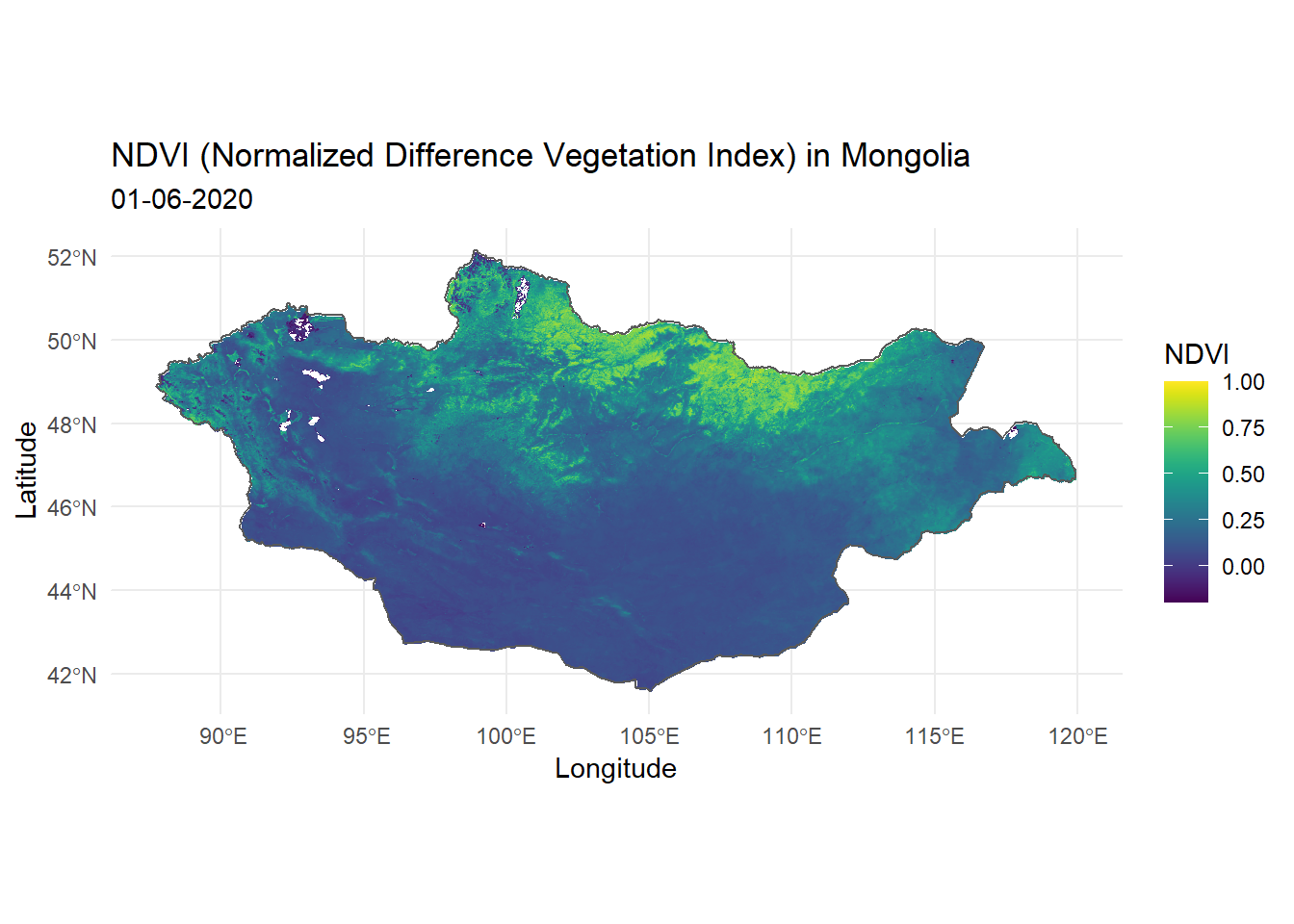
The following example uses the leaflet() function from the leaflet package to visualise the downloaded NDVI (Normalized Difference Vegetation Index) of Mongolia.
# install.packages("leaflet")
library(leaflet)

# Defining color palette
pal <- colorNumeric(c("#440154FF", "#238A8DFF", "#FDE725FF"), values(NDVI_raster), na.color = "transparent")

# Visualising using leaflet
leaflet() %>%
  addTiles() %>%
  addRasterImage(NDVI_raster, colors = pal) %>%
  addLegend(
    pal = pal, values = values(NDVI_raster),
    title = "NDVI"
  )
References
MODISwebsite: https://modis.gsfc.nasa.gov/MODIStspvignette: https://cran.r-project.org/web/packages/MODIStsp/vignettes/MODIStsp.htmlMODIStsp vegetation indexdata product page: https://modis.gsfc.nasa.gov/data/dataprod/mod13.php
Last updated: 2023-01-07
Source code: https://github.com/rspatialdata/rspatialdata.github.io/blob/main/vegetation.Rmd
Tutorial was complied using: (click to expand)
## R version 4.0.3 (2020-10-10)
## Platform: x86_64-w64-mingw32/x64 (64-bit)
## Running under: Windows 10 x64 (build 18363)
##
## Matrix products: default
##
## locale:
## [1] LC_COLLATE=English_United States.1252
## [2] LC_CTYPE=English_United States.1252
## [3] LC_MONETARY=English_United States.1252
## [4] LC_NUMERIC=C
## [5] LC_TIME=English_United States.1252
##
## attached base packages:
## [1] stats     graphics  grDevices utils     datasets  methods   base
##
## other attached packages:
##  [1] rgdal_1.5-23              magrittr_2.0.1
##  [3] spocc_1.2.0               cartogram_0.2.2
##  [5] wopr_0.4.6                ggmap_3.0.0
##  [7] osmdata_0.1.5             malariaAtlas_1.0.1
##  [9] ggthemes_4.2.4            here_1.0.1
## [11] MODIStsp_2.0.9            nasapower_4.0.7
## [13] terra_1.5-17              rnaturalearthhires_0.2.0
## [15] rnaturalearth_0.1.0       viridis_0.5.1
## [17] viridisLite_0.3.0         raster_3.5-15
## [19] sp_1.4-5                  sf_1.0-7
## [21] elevatr_0.4.2             kableExtra_1.3.4
## [23] rdhs_0.7.2                DT_0.17
## [25] forcats_0.5.1             stringr_1.4.0
## [27] dplyr_1.0.4               purrr_0.3.4
## [29] readr_2.1.2               tidyr_1.1.4
## [31] tibble_3.1.6              tidyverse_1.3.1
## [33] openair_2.9-1             leaflet_2.1.1
## [35] ggplot2_3.3.5             rgeoboundaries_0.0.0.9000
##
## loaded via a namespace (and not attached):
##   [1] uuid_0.1-4              readxl_1.3.1            backports_1.4.1
##   [4] systemfonts_1.0.4       plyr_1.8.7              selectr_0.4-2
##   [7] lazyeval_0.2.2          splines_4.0.3           storr_1.2.5
##  [10] crosstalk_1.2.0         urltools_1.7.3          digest_0.6.27
##  [13] htmltools_0.5.2         fansi_0.4.2             memoise_2.0.1
##  [16] cluster_2.1.0           gdalUtilities_1.2.1     tzdb_0.3.0
##  [19] modelr_0.1.8            vroom_1.5.7             xts_0.12.1
##  [22] svglite_1.2.3.2         prettyunits_1.1.1       jpeg_0.1-9
##  [25] colorspace_2.0-3        rvest_1.0.2             rappdirs_0.3.3
##  [28] hoardr_0.5.2            haven_2.5.0             xfun_0.30
##  [31] crayon_1.5.1            jsonlite_1.8.0          hexbin_1.28.2
##  [34] progressr_0.10.1        zoo_1.8-8               countrycode_1.2.0
##  [37] glue_1.6.2              gtable_0.3.0            webshot_0.5.2
##  [40] maps_3.4.0              scales_1.1.1            oai_0.3.2
##  [43] DBI_1.1.2               Rcpp_1.0.7              progress_1.2.2
##  [46] units_0.8-0             bit_4.0.4               mapproj_1.2.8
##  [49] rgbif_3.5.2             htmlwidgets_1.5.4       httr_1.4.2
##  [52] RColorBrewer_1.1-2      wk_0.5.0                ellipsis_0.3.2
##  [55] pkgconfig_2.0.3         farver_2.1.0            sass_0.4.0
##  [58] dbplyr_2.1.1            conditionz_0.1.0        utf8_1.1.4
##  [61] crul_1.2.0              tidyselect_1.1.0        labeling_0.4.2
##  [64] rlang_1.0.2             munsell_0.5.0           cellranger_1.1.0
##  [67] tools_4.0.3             cachem_1.0.6            cli_3.2.0
##  [70] generics_0.1.2          broom_0.8.0             evaluate_0.15
##  [73] fastmap_1.1.0           yaml_2.2.1              knitr_1.33
##  [76] bit64_4.0.5             fs_1.5.2                s2_1.0.7
##  [79] RgoogleMaps_1.4.5.3     nlme_3.1-149            whisker_0.4
##  [82] wellknown_0.7.2         xml2_1.3.2              compiler_4.0.3
##  [85] rstudioapi_0.13         curl_4.3.2              png_0.1-7
##  [88] e1071_1.7-4             reprex_2.0.1            bslib_0.3.1
##  [91] stringi_1.5.3           highr_0.9               gdtools_0.2.4
##  [94] lattice_0.20-41         Matrix_1.2-18           classInt_0.4-3
##  [97] vctrs_0.3.8             slippymath_0.3.1        pillar_1.7.0
## [100] lifecycle_1.0.1         triebeard_0.3.0         jquerylib_0.1.4
## [103] data.table_1.14.2       bitops_1.0-7            R6_2.5.0
## [106] latticeExtra_0.6-29     KernSmooth_2.23-17      gridExtra_2.3
## [109] codetools_0.2-16        MASS_7.3-53             assertthat_0.2.1
## [112] rjson_0.2.20            rprojroot_2.0.2         withr_2.5.0
## [115] httpcode_0.3.0          rbison_1.0.0            rvertnet_0.8.0
## [118] ridigbio_0.3.5          mgcv_1.8-33             parallel_4.0.3
## [121] hms_1.1.1               rebird_1.2.0            grid_4.0.3
## [124] rnaturalearthdata_0.1.0 class_7.3-17            rmarkdown_2.11
## [127] packcircles_0.3.4       base64enc_0.1-3         lubridate_1.8.0
Corrections: If you see mistakes or want to suggest additions or modifications, please create an issue on the source repository or submit a pull request Reuse: Text and figures are licensed under Creative Commons Attribution CC BY 4.0.