Elevation data
Data set details
| Data set description: | Elevation data in Switzerland |
| Source: | USGS Elevation Point Query Service and Amazon Web Services Terrain Tiles |
| Details on the retrieved data: | Elevation in Switzerland along with the data on the administrative areas for the same country. |
| Spatial and temporal resolution: | Elevation data with different zoom levels (see details) |
Downloading elevation data with the elevatr package
This tutorial gives you a brief understanding of how to use the elevatr package for a standardized access to the elevation data from the web. The packages uses two endpoints to access its data from:
- USGS Elevation Point Query Service for point elevation data (for United states only).
- Amazon Web Services Terrain Tiles for raster elevation data such as DEM (digital elevation model) (for all global elevation data).
Installing the package
The elevtr package can be directly downloaded from CRAN as follows.
install.packages("elevatr")Loading the elevatr package:
library(elevatr)Functions available
Currently, there are two functions in this package which help users access elevation web services, namely, get_elev_point() and get_elev_raster().
The get_elev_point() function gets the point elevations using the USGS Elevation Point Query Services (for United states only) and AWS Terrain Tiles (for all global elevation data).
- Input: This function accepts a data frame of longitude and latitude values (
xandy), aSpatialPoints/SpatialPointsDataFrame, or a simple feature object (sf). It has a source argumentsrcwhich indicates which API to use, either"eqps"or"aws".
- Output: produces either a
SpatialPointsDataFrameorSimple Feature object, depending on the class of input locations.
The get_elev_point() function can be used as follows:
ll_proj <- "+proj=longlat +ellps=WGS84 +datum=WGS84 +no_defs"
elev <- elevatr::get_elev_point(pt_df, prj = ll_proj)

library(kableExtra)
elev %>%
  kable() %>%
kable_styling(bootstrap_options = c("striped", "hover"))| elevation | elev_units | coords.x1 | coords.x2 |
|---|---|---|---|
| NA | meters | -71.82791 | 40.25963 |
| 243.79 | meters | -71.76843 | 43.05586 |
| 73.74 | meters | -71.37858 | 42.52338 |
| 86.83 | meters | -71.10417 | 42.65332 |
| 391.93 | meters | -71.56750 | 43.91346 |
The get_elev_raster() function helps users get elevation data as a raster from the AWS Open Data Terrain Tiles. The source data are global and also contain the estimations for depth for oceans.
Input: This takes in a data frame of longitude and latitude values (
xandy) or anysporrasterobject. It has azargument to determine the zoom or resolution of the raster (1 to 14). It also has aclipargument to determine clipping of returned DEM. Options are"tile"which is the default value and returns the full tiles,"bbox"which returns the DEM clipped to the bounding box of the original locations, or"locations"if the spatial data in the input locations should be used to clip the DEM.Output: Returns a
rasterobject of the elevation tiles that cover the bounding box of the input spatial data.
We can use the get_elev_raster() function to obtain the elevation data of Switzerland, and plot it together with the country boundaries obtained by using the rgeoboundaries package as follows.
library(rgeoboundaries)
library(sf)
library(raster)
library(ggplot2)
library(viridis)

swiss_bound <- rgeoboundaries::geoboundaries("Switzerland")
elevation_data <- elevatr::get_elev_raster(locations = swiss_bound, z = 9, clip = "locations")


elevation_data <- as.data.frame(elevation_data, xy = TRUE)
colnames(elevation_data)[3] <- "elevation"
# remove rows of data frame with one or more NA's,using complete.cases
elevation_data <- elevation_data[complete.cases(elevation_data), ]

ggplot() +
  geom_raster(data = elevation_data, aes(x = x, y = y, fill = elevation)) +
  geom_sf(data = swiss_bound, color = "white", fill = NA) +
  coord_sf() +
  scale_fill_viridis_c() +
  labs(title = "Elevation in Switzerland", x = "Longitude", y = "Latitude", fill = "Elevation (meters)")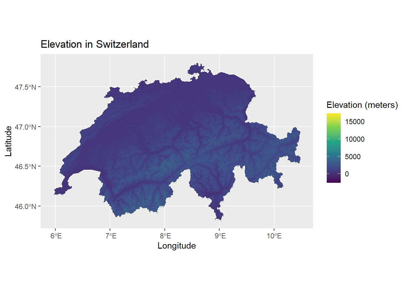
We can also get the different administrative areas of the country Switzerland, by using the ne_states function from the rnaturalearth package. And the get_elev_raster function, you can get the elevation data. The following code does the same:
NOTE: increasing or decreasing the z argument will make the map zoom in and out on the country by setting the appropriate z-axis value.
# install.packages("rnaturlaearth")
# remotes::install_github("ropensci/rnaturalearthhires")

library(rnaturalearth)
library(rnaturalearthhires)

sf_swiss <- ne_states(country = "switzerland", returnclass = "sf")

elevation_1 <- elevatr::get_elev_raster(locations = sf_swiss, z = 7, clip = "locations")
cropped_elev <- crop(elevation_1, sf_swiss)
elevate <- as.data.frame(cropped_elev, xy = TRUE)

colnames(elevate)[3] <- "elevation_value"
elevate <- elevate[complete.cases(elevate), ]

ggplot() +
  # geom_sf(data = st_as_sfc(st_bbox(elevation_1)),color = "grey", fill = "grey",alpha = 0.05) +
  geom_raster(data = elevate, aes(x = x, y = y, fill = elevation_value)) +
  geom_sf(data = sf_swiss, color = "white", fill = NA) +
  coord_sf(xlim = c(5.3, 10.8), ylim = c(45.5, 47.8)) +
  scale_fill_viridis_c() +
  labs(title = "Elevation in Switzerland", x = "Longitude", y = "Latitude", fill = "Elevation (meters)")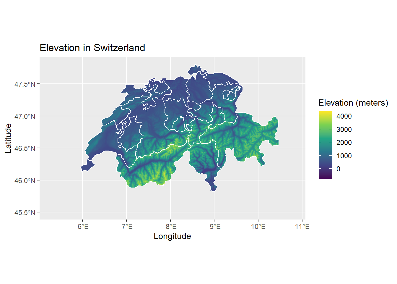
References
elevatrrepository: https://github.com/jhollist/elevatrrgeoboundariespackage: https://gitlab.com/dickoa/rgeoboundariesggplot2package: https://ggplot2.tidyverse.org/
Last updated: 2023-01-07
Source code: https://github.com/rspatialdata/rspatialdata.github.io/blob/main/elevation.Rmd
Tutorial was complied using: (click to expand)
## R version 4.0.3 (2020-10-10)
## Platform: x86_64-w64-mingw32/x64 (64-bit)
## Running under: Windows 10 x64 (build 18363)
##
## Matrix products: default
##
## locale:
## [1] LC_COLLATE=English_United States.1252
## [2] LC_CTYPE=English_United States.1252
## [3] LC_MONETARY=English_United States.1252
## [4] LC_NUMERIC=C
## [5] LC_TIME=English_United States.1252
##
## attached base packages:
## [1] stats     graphics  grDevices utils     datasets  methods   base
##
## other attached packages:
##  [1] rnaturalearthhires_0.2.0  rnaturalearth_0.1.0
##  [3] viridis_0.5.1             viridisLite_0.3.0
##  [5] raster_3.5-15             sp_1.4-5
##  [7] sf_1.0-7                  elevatr_0.4.2
##  [9] kableExtra_1.3.4          rdhs_0.7.2
## [11] DT_0.17                   forcats_0.5.1
## [13] stringr_1.4.0             dplyr_1.0.4
## [15] purrr_0.3.4               readr_2.1.2
## [17] tidyr_1.1.4               tibble_3.1.6
## [19] tidyverse_1.3.1           openair_2.9-1
## [21] leaflet_2.1.1             ggplot2_3.3.5
## [23] rgeoboundaries_0.0.0.9000
##
## loaded via a namespace (and not attached):
##   [1] colorspace_2.0-3    ellipsis_0.3.2      class_7.3-17
##   [4] rgdal_1.5-23        rprojroot_2.0.2     fs_1.5.2
##   [7] httpcode_0.3.0      rstudioapi_0.13     farver_2.1.0
##  [10] hexbin_1.28.2       urltools_1.7.3      bit64_4.0.5
##  [13] fansi_0.4.2         lubridate_1.8.0     xml2_1.3.2
##  [16] codetools_0.2-16    splines_4.0.3       cachem_1.0.6
##  [19] knitr_1.33          jsonlite_1.8.0      broom_0.8.0
##  [22] cluster_2.1.0       dbplyr_2.1.1        png_0.1-7
##  [25] hoardr_0.5.2        mapproj_1.2.8       compiler_4.0.3
##  [28] httr_1.4.2          backports_1.4.1     assertthat_0.2.1
##  [31] Matrix_1.2-18       fastmap_1.1.0       cli_3.2.0
##  [34] s2_1.0.7            prettyunits_1.1.1   htmltools_0.5.2
##  [37] tools_4.0.3         gtable_0.3.0        glue_1.6.2
##  [40] wk_0.5.0            maps_3.4.0          rappdirs_0.3.3
##  [43] Rcpp_1.0.7          cellranger_1.1.0    jquerylib_0.1.4
##  [46] vctrs_0.3.8         crul_1.2.0          svglite_1.2.3.2
##  [49] countrycode_1.2.0   nlme_3.1-149        progressr_0.10.1
##  [52] crosstalk_1.2.0     xfun_0.30           rvest_1.0.2
##  [55] lifecycle_1.0.1     terra_1.5-17        MASS_7.3-53
##  [58] scales_1.1.1        vroom_1.5.7         hms_1.1.1
##  [61] slippymath_0.3.1    parallel_4.0.3      RColorBrewer_1.1-2
##  [64] yaml_2.2.1          curl_4.3.2          gridExtra_2.3
##  [67] memoise_2.0.1       gdtools_0.2.4       sass_0.4.0
##  [70] triebeard_0.3.0     latticeExtra_0.6-29 stringi_1.5.3
##  [73] highr_0.9           e1071_1.7-4         storr_1.2.5
##  [76] systemfonts_1.0.4   rlang_1.0.2         pkgconfig_2.0.3
##  [79] evaluate_0.15       lattice_0.20-41     htmlwidgets_1.5.4
##  [82] labeling_0.4.2      bit_4.0.4           tidyselect_1.1.0
##  [85] here_1.0.1          magrittr_2.0.1      R6_2.5.0
##  [88] generics_0.1.2      DBI_1.1.2           pillar_1.7.0
##  [91] haven_2.5.0         withr_2.5.0         mgcv_1.8-33
##  [94] units_0.8-0         modelr_0.1.8        crayon_1.5.1
##  [97] KernSmooth_2.23-17  utf8_1.1.4          tzdb_0.3.0
## [100] rmarkdown_2.11      progress_1.2.2      jpeg_0.1-9
## [103] grid_4.0.3          readxl_1.3.1        webshot_0.5.2
## [106] reprex_2.0.1        digest_0.6.27       classInt_0.4-3
## [109] munsell_0.5.0       bslib_0.3.1
Corrections: If you see mistakes or want to suggest additions or modifications, please create an issue on the source repository or submit a pull request Reuse: Text and figures are licensed under Creative Commons Attribution CC BY 4.0.