Administrative Boundaries
Data set details
| Data set description: | Administrative boundaries for different countries |
| Source: | geoBoundaries |
| Details on the retrieved data: | Data on different levels of administrative boundaries for countries such as Nigeria and Chad. |
| Spatial and temporal resolution: | World administrative boundaries. |
Downloading administrative boundaries of countries with rgeoboundaries
The rgeoboundaries package is a client for the geoBoundaries API, providing country political administrative boundaries. This tutorial takes you through the steps of downloading administrative boundaries of countries using the rgeoboundaries package and visualising them using the ggplot2 package.
Installing rgeoboundaries
The rgeoboundaries package can be downloaded from GitHub using the remotes package which allows easy installation of R packages from remote repositories such as GitHub. We install and load the remotes package and use it to install the rgeoboundaries package from GitHub as follows.
# install.packages("remotes")
library(remotes)
remotes::install_github("wmgeolab/rgeoboundaries")
Administrative boundaries of a single country
To download boundaries of countries we use the geoboundaries() function of rgeoboundaries. For example, we can download the administrative boundary of Nigeria and assign it to a variable called nigeria_boundary as follows.
library(rgeoboundaries)
nigeria_boundary <- geoboundaries("Nigeria")
The ggplot2 package can be used to plot the administrative boundaries downloaded. ggplot2 allows us to easily visualise simple feature objects using the geom_sf() function and can be used to plot the administrative boundary of Nigeria as follows.
# install.packages("ggplot2")
library(ggplot2)
ggplot(data = nigeria_boundary) +
  geom_sf()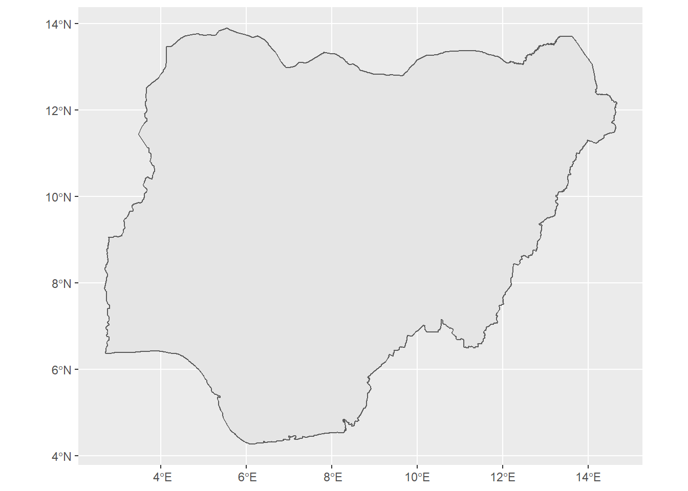
Administrative boundaries of multiple countries
We can also download the boundaries of multiple countries together by including the names of countries as a vector. See how the boundaries of Nigeria and Chad are downloaded below.
nigeria_chad_boundaries <- geoboundaries(c("Nigeria", "Chad"))ggplot(data = nigeria_chad_boundaries) +
geom_sf()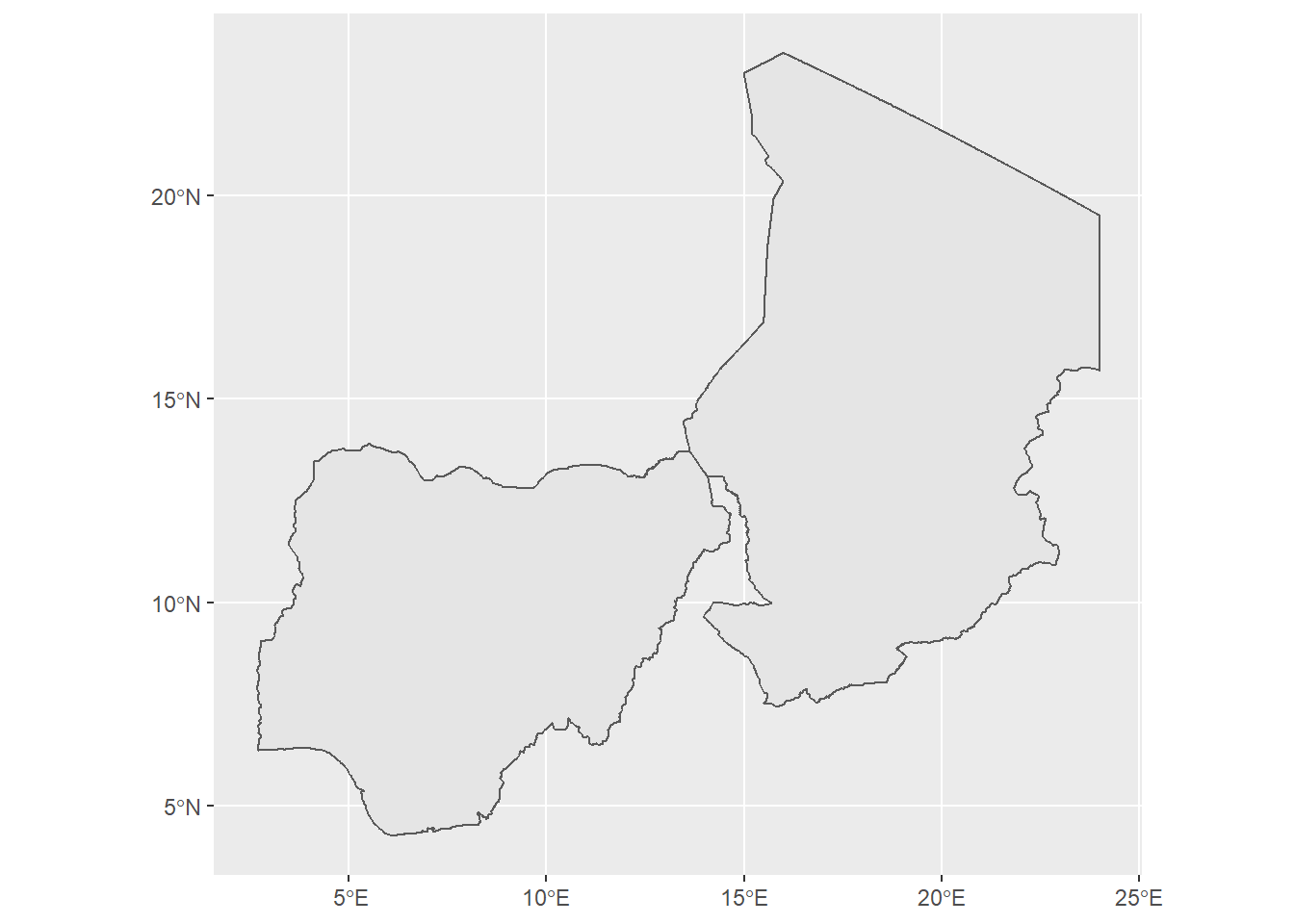
Different levels of administrative boundaries
If available, lower levels of administrative boundaries in countries can be downloaded too. We just have to pass the administrative level as an argument in the geoboundaries() function. Administrative level 1 (“adm1”) is the highest level, while administrative level 5 (“adm5”) is the lowest. This means the country will be further sub-divided into administrative divisions as the Administrative level progresses from 1 to 5. See how the first and second administrative level boundaries of Nigeria and Chad are downloaded below.
# downloading administrative level 1 boundaries
nigeria_chad_admlvl1_boundaries <- geoboundaries(c("Nigeria", "Chad"), "adm1")
ggplot(data = nigeria_chad_admlvl1_boundaries) +
geom_sf()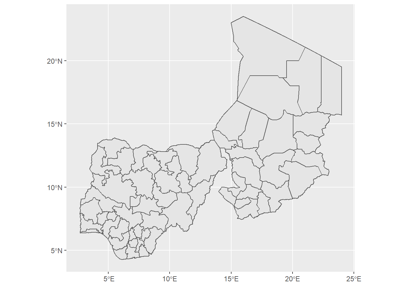
# downloading administrative level 2 boundaries
nigeria_chad_admlvl2_boundaries <- geoboundaries(c("Nigeria", "Chad"), "adm2")
ggplot(data = nigeria_chad_admlvl2_boundaries) +
geom_sf()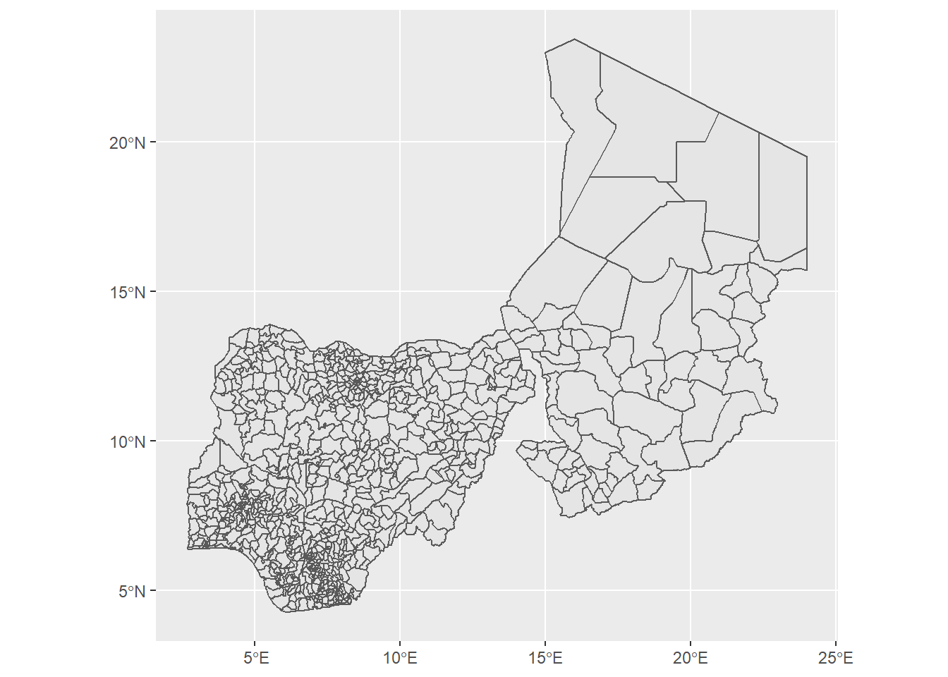
Understanding the downloaded data
If we print out the downloaded administrative boundary of Nigeria, we will see that the downloaded boundary is a simple feature collection with 1 feature and 5 fields. A feature is thought of as a single object, Nigeria in this case. The fields are thought of as the geometrical attributes included about each feature; shapeName, shapeISO, shapeID, shapeGroup and shapeType in the above object.
nigeria_boundary## Simple feature collection with 1 feature and 5 fields
## Geometry type: MULTIPOLYGON
## Dimension: XY
## Bounding box: xmin: 2.668432 ymin: 4.277144 xmax: 14.67808 ymax: 13.90103
## Geodetic CRS: WGS 84
## shapeName shapeISO shapeID shapeGroup shapeType
## 1 Nigeria NGA NGA-ADM0-1590546715-B1 NGA ADM0
## geometry
## 1 MULTIPOLYGON (((5.746892 4....The simple feature object retrieved with the boundaries of Nigeria and Chad is a simple feature collection with 2 features and 5 fields. The 2 features will refer to the two countries (Nigeria and Chad), and the features will be the geometrical attributes of each feature.
nigeria_chad_boundaries## Simple feature collection with 2 features and 5 fields
## Geometry type: GEOMETRY
## Dimension: XY
## Bounding box: xmin: 2.668432 ymin: 4.277144 xmax: 24 ymax: 23.4975
## Geodetic CRS: WGS 84
## shapeName shapeISO shapeID shapeGroup shapeType
## 1 Nigeria NGA NGA-ADM0-1590546715-B1 NGA ADM0
## 2 Chad TCD TCD-ADM0-1590546715-B1 TCD ADM0
## geometry
## 1 MULTIPOLYGON (((5.746892 4....
## 2 POLYGON ((23.99944 15.79972...Similarly, downloads of administrative level 1 (nigeria_chad_admlvl1_boundaries) and 2 (nigeria_chad_admlvl2_boundaries) boundaries of Nigeria and Chad will result in simple feature objects with 60 and 843 features respectively. Here each feature will be a single administrative division. The number of administrative divisions increasing as the countries are further sub-divided from administrative level 1 divisions to administrative level 2 divisions.
The shapeName field of the simple feature objects has the names of the administrative divisions. We can create a map with the names of the divisions for Nigeria and Chad using the geom_sf_label() function and setting label = shapeName.
ggplot(data = nigeria_chad_boundaries) +
geom_sf() +
geom_sf_label(aes(label = shapeName))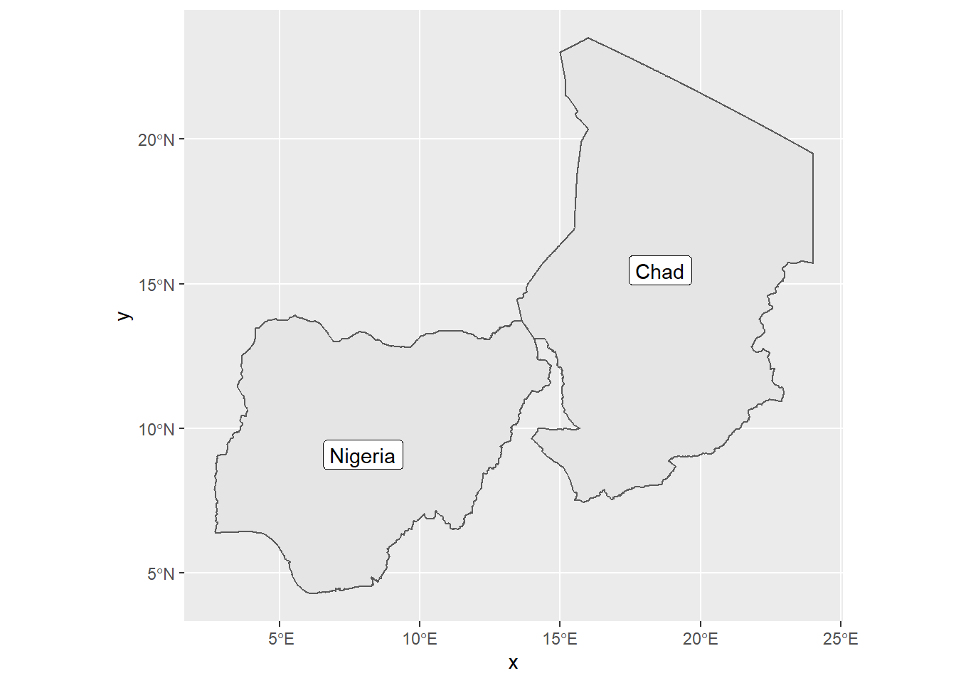
Labelling the administrative divisions also automatically labelled the axes as x and y. If we want to change these axis labels, we can use xlab() and ylab() functions. We can also use the ggtitle() function to add a title to the plot.
ggplot(data = nigeria_chad_boundaries) +
  geom_sf() +
geom_sf_label(aes(label = shapeName)) +
xlab("Longitude") +
ylab("Latitude") +
ggtitle("Nigeria and Chad boundaries")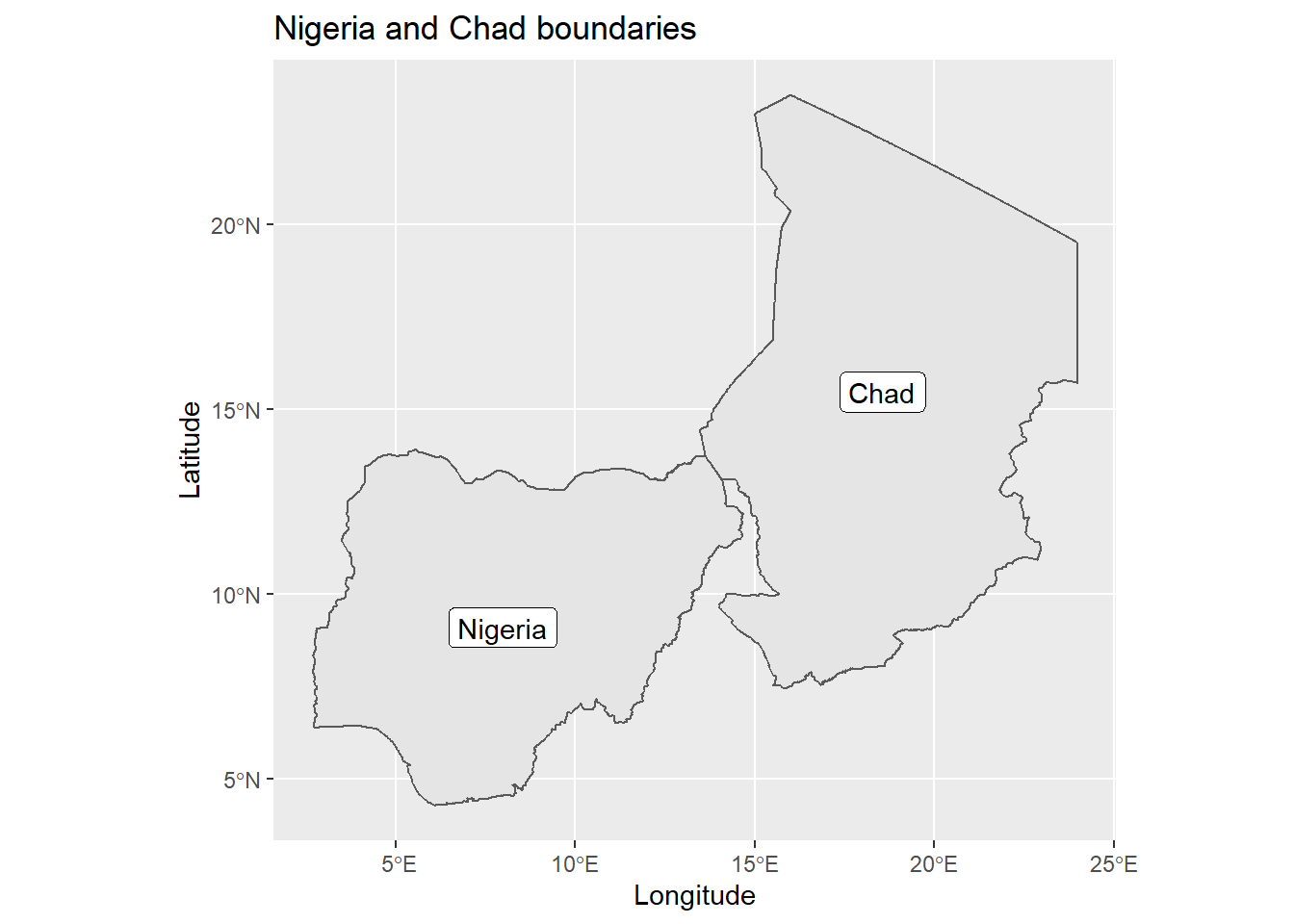
Examples
The following is an example on how to use the rgeoboundaries package to download administrative boundaries and ggplot2 to visualise them.
# remotes::install_github("wmgeolab/rgeoboundaries")
# install.packages("ggplot2")
library(rgeoboundaries)
library(ggplot2)

# Country boundaries of Nigeria and Chad
nigeria_chad_boundaries <- geoboundaries(c("Nigeria", "Chad"))
ggplot(data = nigeria_chad_boundaries) +
  geom_sf() +
  geom_sf_label(aes(label = shapeName)) +
  xlab("Longitude") +
  ylab("Latitude") +
  ggtitle("Country boundaries")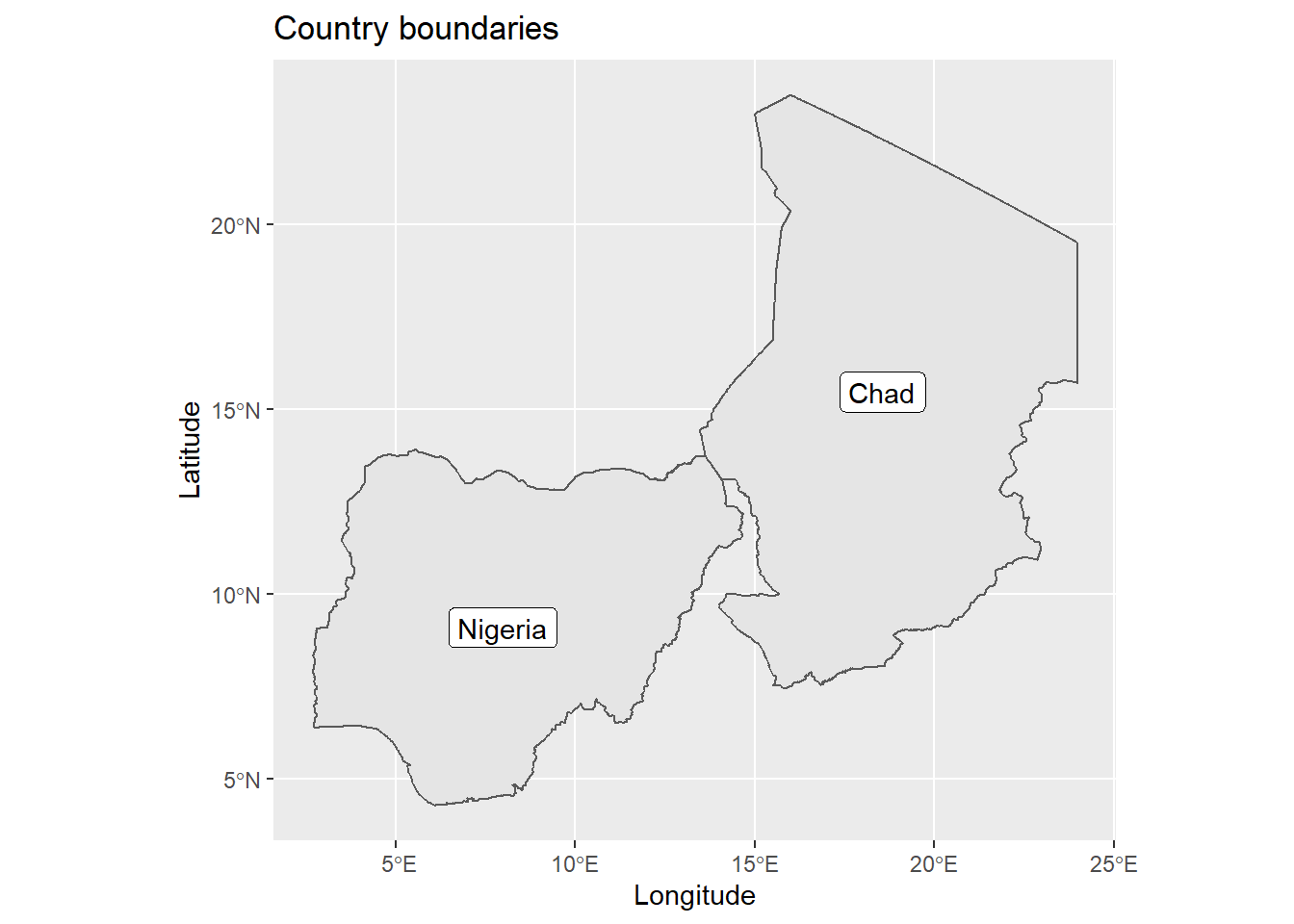
# Administrative Level 1 boundaries of Nigeria and Chad
nigeria_chad_admlvl1_boundaries <- geoboundaries(c("Nigeria", "Chad"), "adm1")
ggplot(data = nigeria_chad_admlvl1_boundaries) +
  geom_sf() +
  ggtitle("Administrative Level 1 boundaries")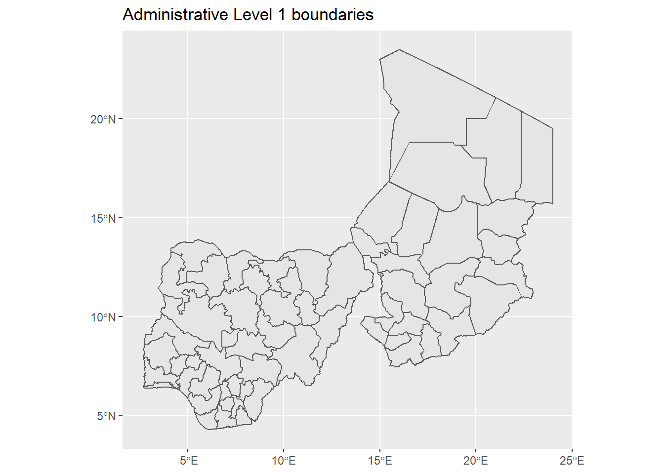
The next example uses the rgeoboundaries package to download administrative boundaries and leaflet to visualise them interactively.
# remotes::install_github("wmgeolab/rgeoboundaries")
# install.packages("leaflet")
library(rgeoboundaries)
library(leaflet)

# Country boundaries of Nigeria and Chad
nigeria_chad_boundaries <- geoboundaries(c("Nigeria", "Chad"))

nigeria_chad_boundaries %>%
  leaflet() %>%
  addTiles() %>%
  addPolygons(label = nigeria_chad_boundaries$shapeName)
# Administrative Level 1 boundaries of Nigeria and Chad
nigeria_chad_admlvl1_boundaries <- geoboundaries(c("Nigeria", "Chad"), "adm1")
nigeria_chad_admlvl1_boundaries %>%
leaflet() %>%
addTiles() %>%
addPolygons(label = nigeria_chad_admlvl1_boundaries$shapeName)References
rgeoboundariesrepository: https://github.com/wmgeolab/rgeoboundaries
ggplot2package: https://ggplot2.tidyverse.org/
Last updated: 2023-01-07
Source code: https://github.com/rspatialdata/rspatialdata.github.io/blob/main/admin_boundaries.Rmd
Tutorial was complied using: (click to expand)
## R version 4.0.3 (2020-10-10)
## Platform: x86_64-w64-mingw32/x64 (64-bit)
## Running under: Windows 10 x64 (build 18363)
##
## Matrix products: default
##
## locale:
## [1] LC_COLLATE=English_United States.1252
## [2] LC_CTYPE=English_United States.1252
## [3] LC_MONETARY=English_United States.1252
## [4] LC_NUMERIC=C
## [5] LC_TIME=English_United States.1252
##
## attached base packages:
## [1] stats     graphics  grDevices utils     datasets  methods   base
##
## other attached packages:
## [1] leaflet_2.1.1             ggplot2_3.3.5
## [3] rgeoboundaries_0.0.0.9000
##
## loaded via a namespace (and not attached):
##  [1] Rcpp_1.0.7         countrycode_1.2.0  class_7.3-17       assertthat_0.2.1
##  [5] digest_0.6.27      utf8_1.1.4         R6_2.5.0           evaluate_0.15
##  [9] e1071_1.7-4        highr_0.9          pillar_1.7.0       rlang_1.0.2
## [13] curl_4.3.2         rstudioapi_0.13    jquerylib_0.1.4    rmarkdown_2.11
## [17] urltools_1.7.3     stringr_1.4.0      htmlwidgets_1.5.4  triebeard_0.3.0
## [21] munsell_0.5.0      compiler_4.0.3     xfun_0.30          pkgconfig_2.0.3
## [25] htmltools_0.5.2    tidyselect_1.1.0   tibble_3.1.6       httpcode_0.3.0
## [29] fansi_0.4.2        crayon_1.5.1       dplyr_1.0.4        hoardr_0.5.2
## [33] withr_2.5.0        sf_1.0-7           wk_0.5.0           rappdirs_0.3.3
## [37] crul_1.2.0         grid_4.0.3         jsonlite_1.8.0     gtable_0.3.0
## [41] lifecycle_1.0.1    DBI_1.1.2          magrittr_2.0.1     units_0.8-0
## [45] scales_1.1.1       KernSmooth_2.23-17 cli_3.2.0          stringi_1.5.3
## [49] cachem_1.0.6       farver_2.1.0       bslib_0.3.1        ellipsis_0.3.2
## [53] generics_0.1.2     vctrs_0.3.8        s2_1.0.7           tools_4.0.3
## [57] glue_1.6.2         purrr_0.3.4        crosstalk_1.2.0    fastmap_1.1.0
## [61] yaml_2.2.1         colorspace_2.0-3   classInt_0.4-3     memoise_2.0.1
## [65] knitr_1.33         sass_0.4.0
Corrections: If you see mistakes or want to suggest additions or modifications, please create an issue on the source repository or submit a pull request Reuse: Text and figures are licensed under Creative Commons Attribution CC BY 4.0.