Rainfall
Data set details
| Data set description: | Rainfall data worldwide and in China |
| Source: | NASA POWER: The POWER Project |
| Details on the retrieved data: | Monthly and yearly rainfall in Australia. |
| Spatial and temporal resolution: | Hourly, daily, monthly, or yearly data for regions defined by the lonlat parameter. Each cell corresponds to 1/2 x 1/2 degree. |
Downloading rainfall data with nasapower
The nasapower package aims at making it quick and easy to automate downloading NASA POWER (NASA Prediction of Worldwide Energy Resource) global meteorology, surface solar energy and climatology data.
Installing nasapower package
The nasapower package can be directly downloaded from CRAN as follows.
install.packages("nasapower")Loading the nasapower package:
library(nasapower)Using get_power() to fetch data
The get_power() function has five arguments and returns a data frame with a metadata header in the current R session. It has the following arguments:
pars: character vector of solar, meteorological or climatology parameters to download.community: character vector providing community name. Supported values are"AG","SB"or"RE".
"AG": provides access to the agroclimatology archive, which contains industry-friendly parameters for input to crop models.
"SB": provides access to the sustainable buildings archive, which contains parameters for the building community.
"RE": provides access to the renewable energy archive, which contains parameters very specific to assist in the design of solar and wind powered renewable energy systems.
temporal_api: temporal API end-point for data being queried. Supported values are"HOURLY","DAILY","MONTHLY", or"CLIMATOLOGY".
"HOURLY": hourly average of pars by hour, day, month and year.
"DAILY": daily average of pars by day, month and year.
"MONTHLY": monthly average of pars by month and year.
"CLIMATOLOGY": provide parameters as 22-year climatologies (solar) and 30-year climatologies (meteorology); the period climatology and monthly average, maximum, and/or minimum values.
lonlat: numeric vector of geographic coordinates for a cell or region or"GLOBAL"for global coverage.
For single point supply a length-two numeric vector giving the decimal degree longitude and latitude in that order for the data to download.
For regional coverage supply a length-four numeric as lower left (lon, lat) and upper right (lon, lat) coordinates as lonlat = c(xmin, ymin, ymax, ymax)
dates: start and end dates. If only one date is provided, it will be treated as both the start and the end date and only a day’s values will be returned. This argument should not be used whentemporal_apiis set to"CLIMATOLOGY".
To know the different weather values from POWER provided within this function, type ?get_power, and in the arguments section, click on the highlighted parameters, which goes to a page which has all the available parameters.
To download rainfall, we use the pars = "PRECTOTCORR".
Fetching daily data for single point
data <- get_power(
  community = "RE",
  lonlat = c(134.489563, -25.734968),
  dates = c("2000-01-01", "2000-05-01"),
  temporal_api = "DAILY",
  pars = "PRECTOTCORR"
)

data %>% datatable(extensions = c("Scroller", "FixedColumns"), options = list(
  deferRender = TRUE,
  scrollY = 350,
  scrollX = 350,
  dom = "t",
  scroller = TRUE,
  fixedColumns = list(leftColumns = 3)
))
Fetching daily data for an area
daily_area <- get_power(
  community = "AG",
  lonlat = c(150.5, -28.5, 153.5, -25.5),
  pars = "PRECTOTCORR",
  dates = c("2004-09-19", "2004-09-29"),
  temporal_api = "DAILY"
)

daily_area %>% datatable(extensions = c("Scroller", "FixedColumns"), options = list(
  deferRender = TRUE,
  scrollY = 350,
  scrollX = 350,
  dom = "t",
  scroller = TRUE,
  fixedColumns = list(leftColumns = 3)
))
Fetching climatology data
Using lonlat equivalent to Australia, we will set temporal_api = "CLIMATOLOGY". Since the maximum processed area is 4.5 x 4.5 degrees (100 points), we will do this in step-by-step.
flag <- 1
for (i in seq(110, 150, 5)) {
  for (j in seq(-40, -10, 5)) {
    climate_avg_temp <- get_power(community = "AG",
                                  pars = "PRECTOTCORR",
                                  lonlat = c(i, (j - 5), (i + 5), j),
                                  temporal_api = "CLIMATOLOGY")
    if (flag == 1) {
      climate_avg <- climate_avg_temp
      flag <- 0
    } else{
      climate_avg <- rbind(climate_avg, climate_avg_temp)
    }
  }
}

climate_avg %>% datatable(extensions = c("Scroller", "FixedColumns"), options = list(
  deferRender = TRUE,
  scrollY = 350,
  scrollX = 350,
  dom = "t",
  scroller = TRUE,
  fixedColumns = list(leftColumns = 3)
))
Next, we will plot the retrieved data.
Creating a map of annual rainfall using all data retrieved
library(rnaturalearth)
library(raster)

# Getting world map
map <- ne_countries(country = 'australia', returnclass = "sf")

# Converting data to raster
r <- rasterFromXYZ(climate_avg[, c("LON", "LAT", "ANN")])

# Converting the raster into a data.frame
r_df <- as.data.frame(r, xy = TRUE, na.rm = TRUE)

# Plot
ggplot() +
  geom_raster(data = r_df, aes(x = x, y = y, fill = ANN)) +
  geom_sf(data = map, inherit.aes = FALSE, fill = NA) +
  scale_fill_viridis() +
  labs(
    title = "Rainfall in inches",
    fill = "Annual Rainfall",
    subtitle = "Annual rainfall in Australia"
  ) +
  labs(x = "Longitude", y = "Latitude")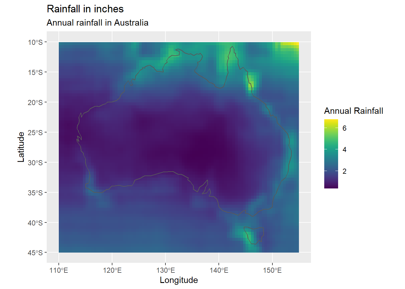
Creating maps of monthly rainfall
r <- list()
for (k in colnames(climate_avg)[-c(1:3, 16)]) {
  r[[k]] <- rasterFromXYZ(climate_avg[, c("LON", "LAT", k)])
}
r <- stack(r)
plot(r, asp = 1)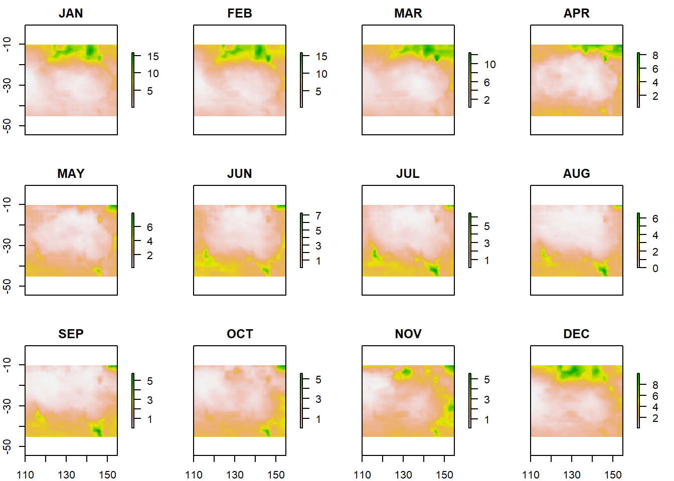
References
nasapowerpackage: https://github.com/ropensci/nasapowerNASAPOWER project: https://power.larc.nasa.gov/
Last updated: 2023-01-07
Source code: https://github.com/rspatialdata/rspatialdata.github.io/blob/main/rainfall.Rmd
Tutorial was complied using: (click to expand)
## R version 4.0.3 (2020-10-10)
## Platform: x86_64-w64-mingw32/x64 (64-bit)
## Running under: Windows 10 x64 (build 18363)
##
## Matrix products: default
##
## locale:
## [1] LC_COLLATE=English_United States.1252
## [2] LC_CTYPE=English_United States.1252
## [3] LC_MONETARY=English_United States.1252
## [4] LC_NUMERIC=C
## [5] LC_TIME=English_United States.1252
##
## attached base packages:
## [1] stats     graphics  grDevices utils     datasets  methods   base
##
## other attached packages:
##  [1] cartogram_0.2.2           wopr_0.4.6
##  [3] ggmap_3.0.0               osmdata_0.1.5
##  [5] malariaAtlas_1.0.1        ggthemes_4.2.4
##  [7] here_1.0.1                MODIStsp_2.0.9
##  [9] nasapower_4.0.7           terra_1.5-17
## [11] rnaturalearthhires_0.2.0  rnaturalearth_0.1.0
## [13] viridis_0.5.1             viridisLite_0.3.0
## [15] raster_3.5-15             sp_1.4-5
## [17] sf_1.0-7                  elevatr_0.4.2
## [19] kableExtra_1.3.4          rdhs_0.7.2
## [21] DT_0.17                   forcats_0.5.1
## [23] stringr_1.4.0             dplyr_1.0.4
## [25] purrr_0.3.4               readr_2.1.2
## [27] tidyr_1.1.4               tibble_3.1.6
## [29] tidyverse_1.3.1           openair_2.9-1
## [31] leaflet_2.1.1             ggplot2_3.3.5
## [33] rgeoboundaries_0.0.0.9000
##
## loaded via a namespace (and not attached):
##   [1] readxl_1.3.1        backports_1.4.1     systemfonts_1.0.4
##   [4] plyr_1.8.7          selectr_0.4-2       splines_4.0.3
##   [7] storr_1.2.5         crosstalk_1.2.0     urltools_1.7.3
##  [10] digest_0.6.27       htmltools_0.5.2     fansi_0.4.2
##  [13] magrittr_2.0.1      memoise_2.0.1       cluster_2.1.0
##  [16] gdalUtilities_1.2.1 tzdb_0.3.0          modelr_0.1.8
##  [19] vroom_1.5.7         xts_0.12.1          svglite_1.2.3.2
##  [22] prettyunits_1.1.1   jpeg_0.1-9          colorspace_2.0-3
##  [25] rvest_1.0.2         rappdirs_0.3.3      hoardr_0.5.2
##  [28] haven_2.5.0         xfun_0.30           rgdal_1.5-23
##  [31] crayon_1.5.1        jsonlite_1.8.0      hexbin_1.28.2
##  [34] progressr_0.10.1    zoo_1.8-8           countrycode_1.2.0
##  [37] glue_1.6.2          gtable_0.3.0        webshot_0.5.2
##  [40] maps_3.4.0          scales_1.1.1        DBI_1.1.2
##  [43] Rcpp_1.0.7          progress_1.2.2      units_0.8-0
##  [46] bit_4.0.4           mapproj_1.2.8       htmlwidgets_1.5.4
##  [49] httr_1.4.2          RColorBrewer_1.1-2  wk_0.5.0
##  [52] ellipsis_0.3.2      pkgconfig_2.0.3     farver_2.1.0
##  [55] sass_0.4.0          dbplyr_2.1.1        utf8_1.1.4
##  [58] crul_1.2.0          tidyselect_1.1.0    labeling_0.4.2
##  [61] rlang_1.0.2         munsell_0.5.0       cellranger_1.1.0
##  [64] tools_4.0.3         cachem_1.0.6        cli_3.2.0
##  [67] generics_0.1.2      broom_0.8.0         evaluate_0.15
##  [70] fastmap_1.1.0       yaml_2.2.1          knitr_1.33
##  [73] bit64_4.0.5         fs_1.5.2            s2_1.0.7
##  [76] RgoogleMaps_1.4.5.3 nlme_3.1-149        xml2_1.3.2
##  [79] compiler_4.0.3      rstudioapi_0.13     curl_4.3.2
##  [82] png_0.1-7           e1071_1.7-4         reprex_2.0.1
##  [85] bslib_0.3.1         stringi_1.5.3       highr_0.9
##  [88] gdtools_0.2.4       lattice_0.20-41     Matrix_1.2-18
##  [91] classInt_0.4-3      vctrs_0.3.8         slippymath_0.3.1
##  [94] pillar_1.7.0        lifecycle_1.0.1     triebeard_0.3.0
##  [97] jquerylib_0.1.4     data.table_1.14.2   bitops_1.0-7
## [100] R6_2.5.0            latticeExtra_0.6-29 KernSmooth_2.23-17
## [103] gridExtra_2.3       codetools_0.2-16    MASS_7.3-53
## [106] assertthat_0.2.1    rjson_0.2.20        rprojroot_2.0.2
## [109] withr_2.5.0         httpcode_0.3.0      mgcv_1.8-33
## [112] parallel_4.0.3      hms_1.1.1           grid_4.0.3
## [115] class_7.3-17        rmarkdown_2.11      packcircles_0.3.4
## [118] lubridate_1.8.0
Corrections: If you see mistakes or want to suggest additions or modifications, please create an issue on the source repository or submit a pull request Reuse: Text and figures are licensed under Creative Commons Attribution CC BY 4.0.