Humidity
| Data set description: | Humidity data worldwide and in Australia |
| Source: | NASA POWER: The POWER Project |
| Details on the retrieved data: | Monthly and yearly relative humidity in Northern Territory and Western Australia (Australia). |
| Spatial and temporal resolution: | Hourly, daily, monthly, or yearly data for regions defined by the lonlat parameter. Each cell corresponds to 1/2 x 1/2 degree. |
Downloading humidity data with nasapower
The nasapower package aims at making it quick and easy to automate downloading NASA POWER (NASA Prediction of Worldwide Energy Resource) global meteorology, surface solar energy and climatology data.
Here, we will use the nasapower package to retrieve the relative humidity data for specific countries or for the world.
We have also used the nasapower package to retrieve rainfall data here. The rainfall tutorial includes an introduction on the nasapower package and how its functions work.
Installing nasapower package
We can install the package from CRAN and load it as follows.
install.packages("nasapower")library(nasapower)Using get_power() to fetch data
First let us have a look at how to get the daily data for humidity in agriculture. This can be done using the get_power() function.
Fetching daily data for single point
We use get_power() function arguments pars = "RH2M" which means relative humidity at 2 meters, temporal_api = "DAILY", and longlat equal to a single location.
data_RH <- get_power(
  community = "AG",
  lonlat = c(134.489563, -25.734968),
  dates = c("2010-09-23", "2010-12-23"),
  temporal_api = "DAILY",
  pars = "RH2M"
)

data_RH %>% datatable(extensions = c("Scroller", "FixedColumns"), options = list(
  deferRender = TRUE,
  scrollY = 350,
  scrollX = 350,
  dom = "t",
  scroller = TRUE,
  fixedColumns = list(leftColumns = 3)
))
Fetching daily data for an area
daily_humidity <- get_power(
  community = "AG",
  lonlat = c(150, -30, 155, -25),
  pars = "RH2M",
  dates = c("2004-09-19", "2004-09-29"),
  temporal_api = "DAILY"
)

daily_humidity %>% datatable(extensions = c("Scroller", "FixedColumns"), options = list(
  deferRender = TRUE,
  scrollY = 350,
  scrollX = 350,
  dom = "t",
  scroller = TRUE,
  fixedColumns = list(leftColumns = 3)
))
Fetching climatology data
For pars = "RH2M", and as in the rainfall tutorial we will focus on Australia territory and set community = "AG" and temporal_api = "CLIMATOLOGY".
flag <- 1
for (i in seq(110, 150, 5)) {
  for (j in seq(-40, -10, 5)) {
    climate_avg_RH_temp <- get_power(community = "AG",
                                  pars = "RH2M",
                                  lonlat = c(i, (j - 5), (i + 5), j),
                                  temporal_api = "CLIMATOLOGY")
    if (flag == 1) {
      climate_avg_RH <- climate_avg_RH_temp
      flag <- 0
    } else{
      climate_avg_RH <- rbind(climate_avg_RH, climate_avg_RH_temp)
    }
  }
}

climate_avg_RH %>% datatable(extensions = c("Scroller", "FixedColumns"), options = list(
  deferRender = TRUE,
  scrollY = 350,
  scrollX = 350,
  dom = "t",
  scroller = TRUE,
  fixedColumns = list(leftColumns = 3)
))
Creating a map of annual humidity using all data retrieved
library(rnaturalearth)
library(raster)
# Getting world map
map <- ne_countries(country = 'australia', returnclass = "sf")
# Converting data to raster
r <- rasterFromXYZ(climate_avg_RH[, c("LON", "LAT", "ANN")])
# Converting the raster into a data.frame
r_df <- as.data.frame(r, xy = TRUE, na.rm = TRUE)
# Plot
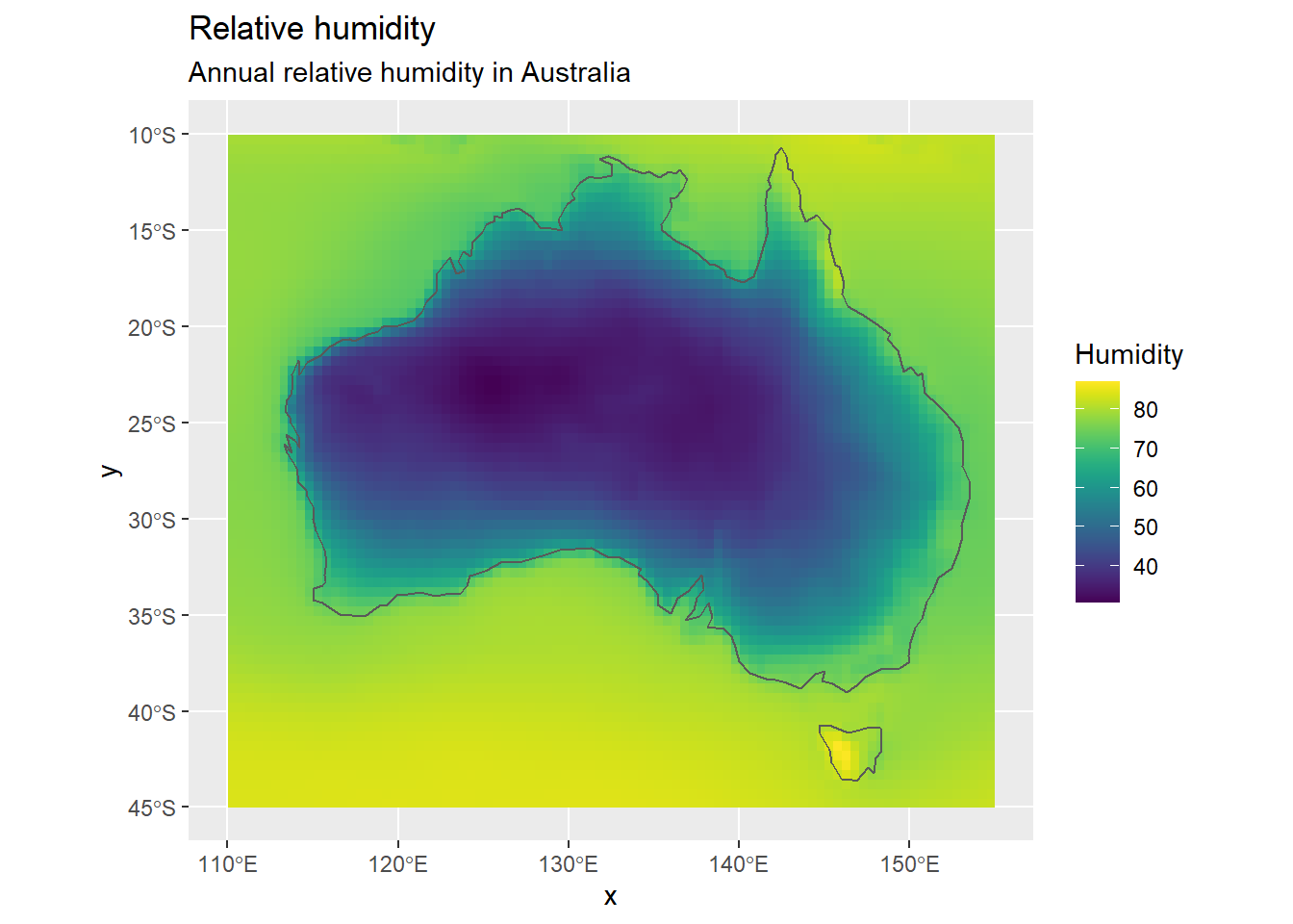
ggplot() +
geom_raster(data = r_df, aes(x = x, y = y, fill = ANN)) +
geom_sf(data = map, inherit.aes = FALSE, fill = NA) +
scale_fill_viridis() +
labs(
title = "Relative humidity",
fill = "Humidity",
subtitle = "Annual relative humidity in Australia"
)
Creating a map of annual humidity using a subset of the data retrieved
library(rnaturalearth)

# Getting map for China
AUS <- ne_states(country = "Australia", returnclass = "sf")

# Getting administrative boundaries for regions
NT <- AUS[AUS$name == "Northern Territory", ]
WA <- AUS[AUS$name == "Western Australia", ]

# Converting data to raster
r <- rasterFromXYZ(climate_avg_RH[, c("LON", "LAT", "ANN")])

# Subset values for the region and converting the raster into a data.frame
rr <- mask(crop(r, NT), NT)
r_df <- as.data.frame(rr, xy = TRUE, na.rm = TRUE)

ggplot() +
  geom_raster(data = r_df, aes(x = x, y = y, fill = ANN)) +
  geom_sf(data = AUS, inherit.aes = FALSE, fill = NA) +
  scale_fill_viridis() +
  theme_minimal() +
  labs(title = "Relative Humidity in Northern Territory, Australia", fill = "Humidity")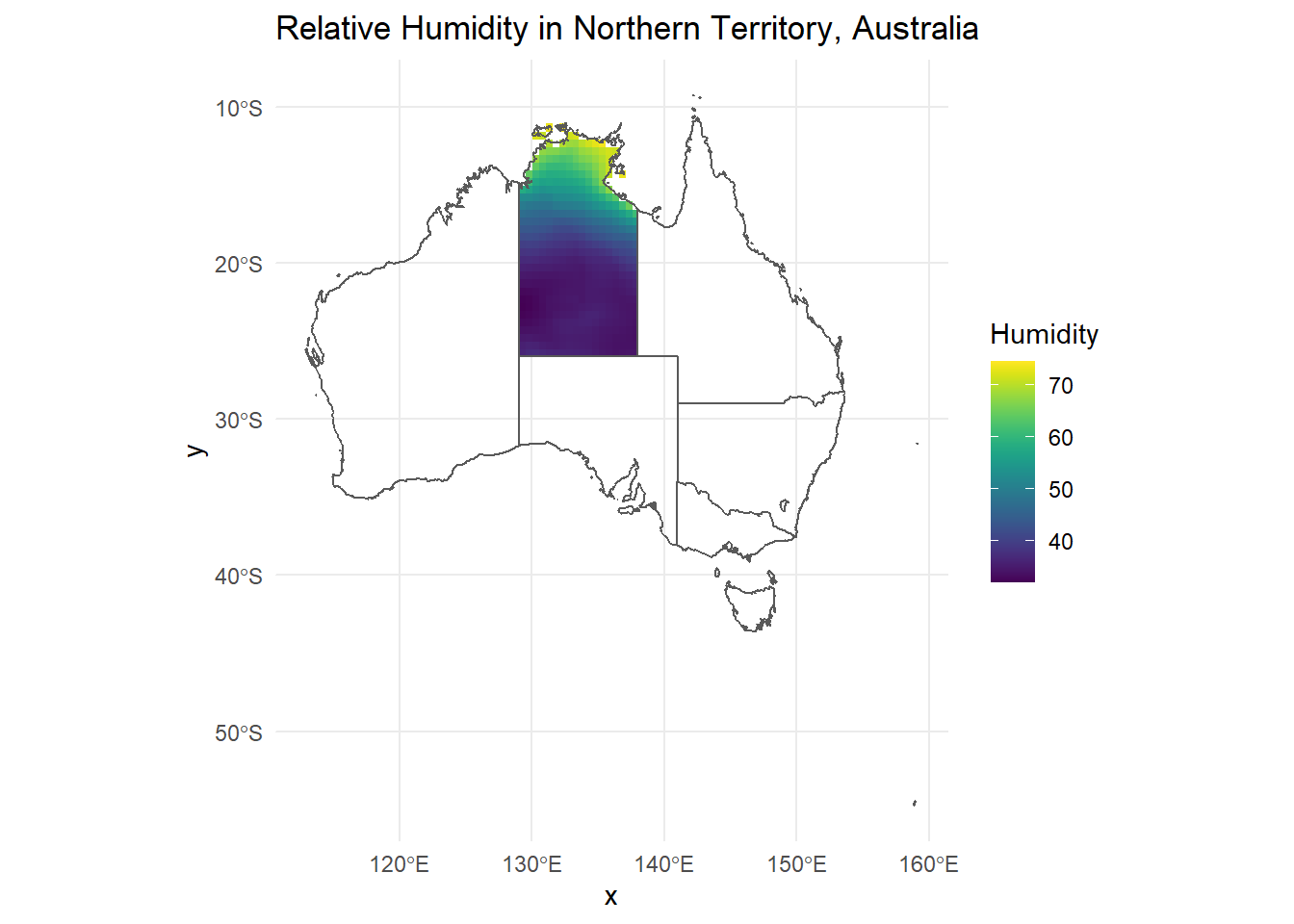
# Subset values for the region and converting the raster into a data.frame
rr <- mask(crop(r, WA), WA)
r_df <- as.data.frame(rr, xy = TRUE, na.rm = TRUE)

ggplot() +
  geom_raster(data = r_df, aes(x = x, y = y, fill = ANN)) +
  geom_sf(data = AUS, inherit.aes = FALSE, fill = NA) +
  scale_fill_viridis() +
  theme_minimal() +
  labs(title = "Relative Humidity in Western Australia, Australia", fill = "Humidity")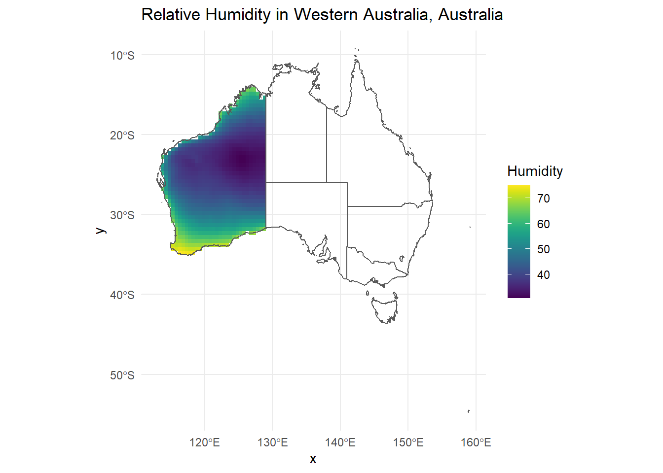
Creating maps of monthly humidity
r <- list()
for (k in colnames(climate_avg_RH)[-c(1:3, 16)]) {
  r[[k]] <- rasterFromXYZ(climate_avg_RH[, c("LON", "LAT", k)])
}
r <- stack(r)
plot(r)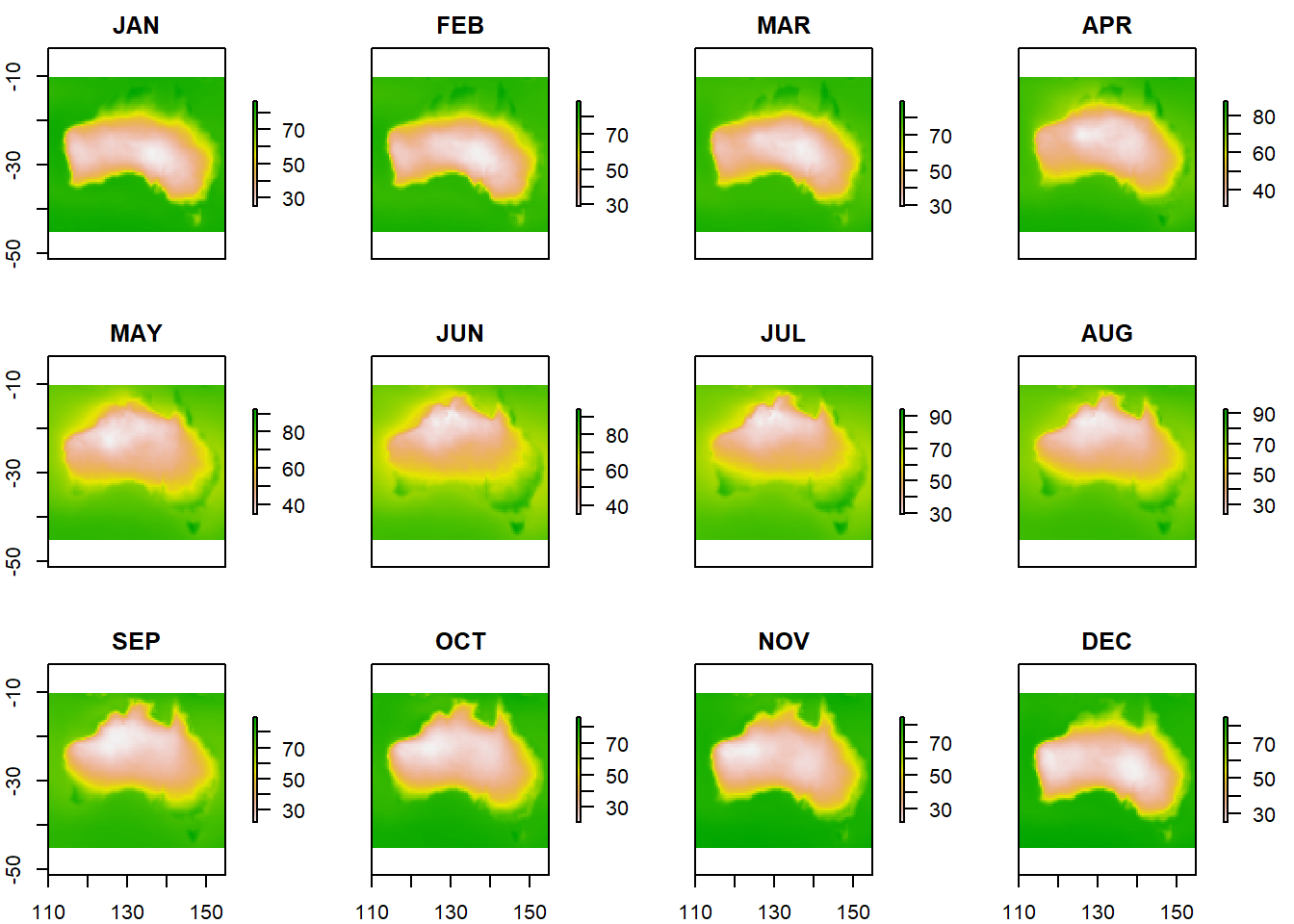
References
nasapowerpackage: https://github.com/ropensci/nasapowerNASAPOWER project: https://power.larc.nasa.gov/
Last updated: 2023-01-07
Source code: https://github.com/rspatialdata/rspatialdata.github.io/blob/main/humidity.Rmd
Tutorial was complied using: (click to expand)
## R version 4.0.3 (2020-10-10)
## Platform: x86_64-w64-mingw32/x64 (64-bit)
## Running under: Windows 10 x64 (build 18363)
##
## Matrix products: default
##
## locale:
## [1] LC_COLLATE=English_United States.1252
## [2] LC_CTYPE=English_United States.1252
## [3] LC_MONETARY=English_United States.1252
## [4] LC_NUMERIC=C
## [5] LC_TIME=English_United States.1252
##
## attached base packages:
## [1] stats     graphics  grDevices utils     datasets  methods   base
##
## other attached packages:
##  [1] nasapower_4.0.7           terra_1.5-17
##  [3] rnaturalearthhires_0.2.0  rnaturalearth_0.1.0
##  [5] viridis_0.5.1             viridisLite_0.3.0
##  [7] raster_3.5-15             sp_1.4-5
##  [9] sf_1.0-7                  elevatr_0.4.2
## [11] kableExtra_1.3.4          rdhs_0.7.2
## [13] DT_0.17                   forcats_0.5.1
## [15] stringr_1.4.0             dplyr_1.0.4
## [17] purrr_0.3.4               readr_2.1.2
## [19] tidyr_1.1.4               tibble_3.1.6
## [21] tidyverse_1.3.1           openair_2.9-1
## [23] leaflet_2.1.1             ggplot2_3.3.5
## [25] rgeoboundaries_0.0.0.9000
##
## loaded via a namespace (and not attached):
##   [1] colorspace_2.0-3    ellipsis_0.3.2      class_7.3-17
##   [4] rgdal_1.5-23        rprojroot_2.0.2     fs_1.5.2
##   [7] httpcode_0.3.0      rstudioapi_0.13     farver_2.1.0
##  [10] hexbin_1.28.2       urltools_1.7.3      bit64_4.0.5
##  [13] fansi_0.4.2         lubridate_1.8.0     xml2_1.3.2
##  [16] codetools_0.2-16    splines_4.0.3       cachem_1.0.6
##  [19] knitr_1.33          jsonlite_1.8.0      broom_0.8.0
##  [22] cluster_2.1.0       dbplyr_2.1.1        png_0.1-7
##  [25] hoardr_0.5.2        mapproj_1.2.8       compiler_4.0.3
##  [28] httr_1.4.2          backports_1.4.1     assertthat_0.2.1
##  [31] Matrix_1.2-18       fastmap_1.1.0       cli_3.2.0
##  [34] s2_1.0.7            prettyunits_1.1.1   htmltools_0.5.2
##  [37] tools_4.0.3         gtable_0.3.0        glue_1.6.2
##  [40] wk_0.5.0            maps_3.4.0          rappdirs_0.3.3
##  [43] Rcpp_1.0.7          cellranger_1.1.0    jquerylib_0.1.4
##  [46] vctrs_0.3.8         crul_1.2.0          svglite_1.2.3.2
##  [49] countrycode_1.2.0   nlme_3.1-149        progressr_0.10.1
##  [52] crosstalk_1.2.0     xfun_0.30           rvest_1.0.2
##  [55] lifecycle_1.0.1     MASS_7.3-53         scales_1.1.1
##  [58] vroom_1.5.7         hms_1.1.1           slippymath_0.3.1
##  [61] parallel_4.0.3      RColorBrewer_1.1-2  yaml_2.2.1
##  [64] curl_4.3.2          gridExtra_2.3       memoise_2.0.1
##  [67] gdtools_0.2.4       sass_0.4.0          triebeard_0.3.0
##  [70] latticeExtra_0.6-29 stringi_1.5.3       highr_0.9
##  [73] e1071_1.7-4         storr_1.2.5         systemfonts_1.0.4
##  [76] rlang_1.0.2         pkgconfig_2.0.3     evaluate_0.15
##  [79] lattice_0.20-41     htmlwidgets_1.5.4   labeling_0.4.2
##  [82] bit_4.0.4           tidyselect_1.1.0    here_1.0.1
##  [85] magrittr_2.0.1      R6_2.5.0            generics_0.1.2
##  [88] DBI_1.1.2           pillar_1.7.0        haven_2.5.0
##  [91] withr_2.5.0         mgcv_1.8-33         units_0.8-0
##  [94] modelr_0.1.8        crayon_1.5.1        KernSmooth_2.23-17
##  [97] utf8_1.1.4          tzdb_0.3.0          rmarkdown_2.11
## [100] progress_1.2.2      jpeg_0.1-9          grid_4.0.3
## [103] readxl_1.3.1        webshot_0.5.2       reprex_2.0.1
## [106] digest_0.6.27       classInt_0.4-3      munsell_0.5.0
## [109] bslib_0.3.1
Corrections: If you see mistakes or want to suggest additions or modifications, please create an issue on the source repository or submit a pull request Reuse: Text and figures are licensed under Creative Commons Attribution CC BY 4.0.