Population

Data set details

Data set description:	Estimated population in Nigeria
Source:	WorldPop Open Population Repository
Details on the retrieved data:	Estimated population in Nigeria for both administrative level 1 and 2 divisions.
Spatial and temporal resolution:	Population data for a list of countries, each divided into smaller regions (administrative levels 1 and 2).

Downloading Population data using wopr

The R package wopr provides access to the WorldPop Open Population Repository and gets estimates of population sizes for specific geographic areas.

Installing wopr

The wopr package can be directly downloaded from the GitHub repository of the package. For this we use the remotes package which allows easy installation of R packages from remote repositories such as GitHub. So we install and load the remotes package and use it to install the wopr package as follows.

# install.packages("remotes")
library(remotes)
remotes::install_github("wpgp/wopr")

Downloading data

To download the population data we first retrieve the WOPR data catalogue to see a list of currently available databases. For this we can use the getCatalogue() function.

library(wopr)

catalogue <- getCatalogue(spatial_query = T)
catalogue

##     country version
## 29      BFA    v1.0
## 36      BFA    v1.1
## 79      COD    v2.0
## 86      COD    v3.0
## 145     GHA    v2.0
## 152     GIN    v1.0
## 214     MOZ    v1.1
## 262     NGA    v1.2
## 269     NGA    v2.0
## 304     SLE    v2.0
## 319     SSD    v2.0
## 377     ZMB    v1.0

Then we simply subset the catalogue for Nigeria (ISO country code NGA) and download the data for the subsetted catalogue selection using the downloadData() function. Note that WOPR uses ISO country codes to abbreviate country names. Also note that downloadData() will not download files larger than 100MB by default unless the maxsize argument is changed (see ?downloadData)

# Select files from the catalogue by subsetting the data frame
selection <- subset(
  catalogue,
  country == "NGA" &
    category == "Population" &
    version == "v1.2"
)

# Download selected files
downloadData(selection)

Understanding the downloaded data

The download will create a folder named ./wopr in your R working directory for the downloaded files, and a spreadsheet with information on the downloaded files will be available at ./wopr/wopr_catalogue.csv. Since we downloaded the population estimates of Nigeria(NGA), zipped data files will be available at ./wopr/NGA/population/v1.2 which will then have to be manually unzipped. The folder structure will look like this:

working directory
└── wopr
    ├── wopr_catalogue.csv
    └── NGA
        └── population
            └── v1.2
                ├── NGA_population_v1_2_admin.zip
                ├── NGA_population_v1_2_gridded.zip
                ├── NGA_population_v1_2_mastergrid.tif
                ├── NGA_population_v1_2_methods.zip
                └── NGA_population_v1_2_README.pdf

Since the zipped file ./wopr/NGA/population/v1.2/NGA_population_v1_2_admin.zip contains population totals for administrative units in Nigeria (i.e. states and local government areas) and shapefiles for the administrative boundaries, we unzip this file and place it in the same directory - after which the folder structure will look like this:

working directory
└── wopr
    ├── wopr_catalogue.csv
    └── NGA
        └── population
            └── v1.2
                ├── NGA_population_v1_2_admin.zip
                ├── ...
                └── NGA_population_v1_2_admin
                  ├── NGA_population_v1_2_admin_level0.csv
                  ├── ...

The unzipped folder (at ./wopr/NGA/population/v1.2/NGA_population_v1_2_admin) will contain multiple .csv files and .shp files containing data on multiple administrative levels of Nigeria, which we will use to visualise the population. The .csv files contain a summary of the distributions of the population estimates, while the .shp files contain vector geospatial data for the respective administrative divisions.

Population of different administrative levels of Nigeria

We use the sf package to read in the downloaded shapefiles into R. We also use the here package to get file paths to the working directory, so that we can simply use relative paths to import files placed within the working directory. First we read in the administrative level 2 data of Nigeria as follows:

# install.packages(c("sf", "here"))
library(sf)
library(here)

admin_level2_shape <- st_read(here::here("wopr/NGA/population/v1.2/NGA_population_v1_2_admin/NGA_population_v1_2_admin_level2_boundaries.shp"))

## Reading layer `NGA_population_v1_2_admin_level2_boundaries' from data source 
##   `C:\rspatialdata.github.io\wopr\NGA\population\v1.2\NGA_population_v1_2_admin\NGA_population_v1_2_admin_level2_boundaries.shp' 
##   using driver `ESRI Shapefile'
## Simple feature collection with 37 features and 17 fields
## Geometry type: MULTIPOLYGON
## Dimension:     XY
## Bounding box:  xmin: 2.6925 ymin: 4.271484 xmax: 14.67797 ymax: 13.88571
## Geodetic CRS:  WGS 84

Then the ggplot2 package can be used to plot the administrative boundaries and visualise the population. The geom_sf() function in the ggplot2 package allows us to easily visualise simple feature objects. We also color the administrative divisions in proportion to its population as follows. Note that wopr provides estimates for the population mean and uncertainty intervals, and we use the variable ‘mean’ to fill in the divisions. The legend on the right of the map describes the color scale used.

# install.packages(c("sf", "ggplot2"))

library(sf)
library(ggplot2)
admin_level2_shape %>%
  ggplot(aes(fill = mean)) +
  geom_sf() +
  scale_fill_continuous(name = "Population")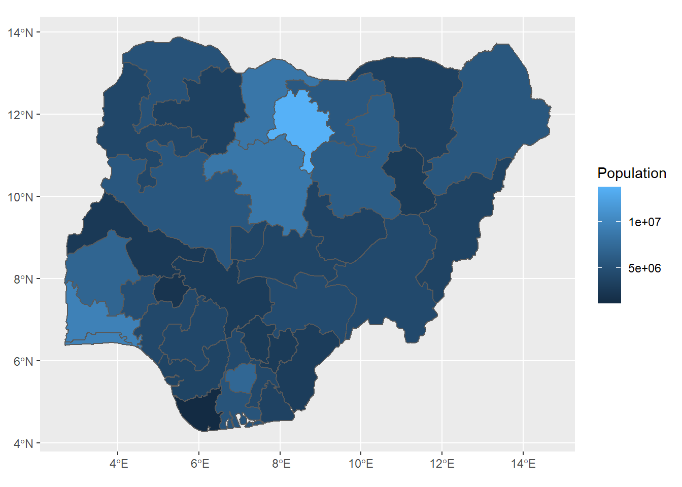

Examples

Choropleth Maps

One of the most common methods of visualising population is through Choropleth maps - which is simply a map with divided geographical areas colored in proportion to a specific variable.

To visualise the population of Nigeria, follow the first few steps of this tutorial to download the population data using the wopr package, unzip the downloaded files and place the files within the working directory. Don’t forget to update the filepaths used in the examples below, to the locations of your data files.

The following example uses the downloaded the population of Nigeria and the sf and ggplot2 packages to visualise the population using a choropleth map. Note how each administrative division in Nigeria has been colored according to its population.

# install.packages(c("sf", "here", "ggplot2"))
library(sf)
library(here)
library(ggplot2)


admin_level2_shape <- st_read(here::here("wopr/NGA/population/v1.2/NGA_population_v1_2_admin/NGA_population_v1_2_admin_level2_boundaries.shp"))

## Reading layer `NGA_population_v1_2_admin_level2_boundaries' from data source 
##   `C:\rspatialdata.github.io\wopr\NGA\population\v1.2\NGA_population_v1_2_admin\NGA_population_v1_2_admin_level2_boundaries.shp' 
##   using driver `ESRI Shapefile'
## Simple feature collection with 37 features and 17 fields
## Geometry type: MULTIPOLYGON
## Dimension:     XY
## Bounding box:  xmin: 2.6925 ymin: 4.271484 xmax: 14.67797 ymax: 13.88571
## Geodetic CRS:  WGS 84

admin_level2_shape %>%
  ggplot(aes(fill = mean)) +
  geom_sf() +
  labs(
    title = "Choropleth map of population in Nigeria",
    subtitle = "Administrative level 2 divisions"
  ) +
  xlab("Longitude") +
  ylab("Latitude") +
  scale_fill_continuous(name = "Population")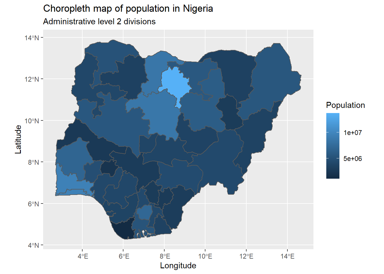

Similarly the administrative level 3 data can also be visualised as follows:

# install.packages(c("sf", "here", "ggplot2"))
library(sf)
library(here)
library(ggplot2)

admin_level3_shape <- st_read(here::here("wopr/NGA/population/v1.2/NGA_population_v1_2_admin/NGA_population_v1_2_admin_level3_boundaries.shp"))

## Reading layer `NGA_population_v1_2_admin_level3_boundaries' from data source 
##   `C:\rspatialdata.github.io\wopr\NGA\population\v1.2\NGA_population_v1_2_admin\NGA_population_v1_2_admin_level3_boundaries.shp' 
##   using driver `ESRI Shapefile'
## Simple feature collection with 774 features and 18 fields
## Geometry type: MULTIPOLYGON
## Dimension:     XY
## Bounding box:  xmin: 2.6925 ymin: 4.271484 xmax: 14.67797 ymax: 13.88571
## Geodetic CRS:  WGS 84

admin_level3_shape %>%
  ggplot(aes(fill = mean)) +
  geom_sf() +
  labs(
    title = "Choropleth map of population in Nigeria",
    subtitle = "Administrative level 3 divisions"
  ) +
  xlab("Longitude") +
  ylab("Latitude") +
  scale_fill_continuous(name = "Population")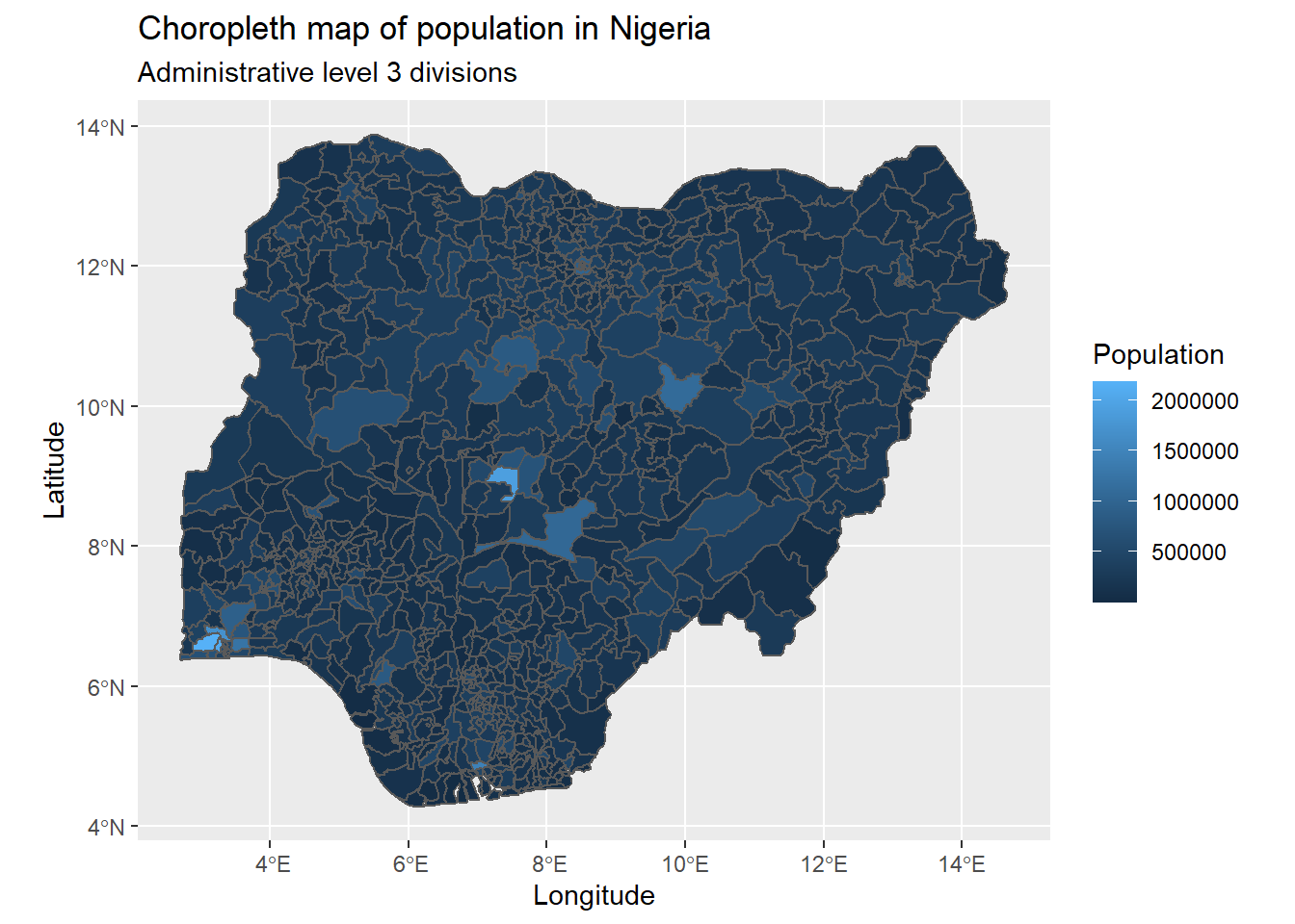

Interactive choropleth maps can also be visualised using the leaflet package.

# install.packages(c("here", "leaflet"))
library(here)
library(leaflet)

admin_level2_shape <- st_read(here::here("wopr/NGA/population/v1.2/NGA_population_v1_2_admin/NGA_population_v1_2_admin_level2_boundaries.shp"))

## Reading layer `NGA_population_v1_2_admin_level2_boundaries' from data source 
##   `C:\rspatialdata.github.io\wopr\NGA\population\v1.2\NGA_population_v1_2_admin\NGA_population_v1_2_admin_level2_boundaries.shp' 
##   using driver `ESRI Shapefile'
## Simple feature collection with 37 features and 17 fields
## Geometry type: MULTIPOLYGON
## Dimension:     XY
## Bounding box:  xmin: 2.6925 ymin: 4.271484 xmax: 14.67797 ymax: 13.88571
## Geodetic CRS:  WGS 84

color_palette <- colorBin("Blues", domain = admin_level2_shape$mean)

admin_level2_shape %>%
  leaflet() %>%
  addTiles() %>%
  addPolygons(
    fillColor = ~ color_palette(mean),
    weight = 2,
    opacity = 1,
    color = "white",
    fillOpacity = 0.7,
    label = admin_level2_shape$statename
  ) %>%
  addLegend(
    pal = color_palette,
    values = ~mean,
    opacity = 0.7,
    title = "Population",
    position = "bottomright"
  )

A downside of choropleth maps is that geographical areas which are bigger in size tend to have a bigger weight on the map, and creates a bias towards that geographical area. To prevent this bias, we can use cartograms.

Cartograms

Another method that can be used to visualise population is by using a cartogram. A cartogram is a map with its geographical regions distorted based on an alternate variable. In a cartogram the area of the geographical regions will be inflated or deflated according to the numeric value of the variable it’s based on.

To visualise the population of Nigeria, follow the first few steps of this tutorial to download the population data using the wopr package, unzip the downloaded files and place the files within the working directory. Don’t forget to update the filepaths used in the examples below, to the locations of your data files.

The following example uses the downloaded population of Nigeria, the cartogram package to create a cartogram based on the population, and the sf and ggplot2 packages to visualise the created cartogram. Note how each administrative division in Nigeria has been colored and resized in proportion to its population.

# install.packages(c("sf", "here", "cartogram", "ggplot2"))
library(sf)
library(here)
library(cartogram)
library(ggplot2)

admin_level2_sf <- st_read(here::here("wopr/NGA/population/v1.2/NGA_population_v1_2_admin/NGA_population_v1_2_admin_level2_boundaries.shp"))

## Reading layer `NGA_population_v1_2_admin_level2_boundaries' from data source 
##   `C:\rspatialdata.github.io\wopr\NGA\population\v1.2\NGA_population_v1_2_admin\NGA_population_v1_2_admin_level2_boundaries.shp' 
##   using driver `ESRI Shapefile'
## Simple feature collection with 37 features and 17 fields
## Geometry type: MULTIPOLYGON
## Dimension:     XY
## Bounding box:  xmin: 2.6925 ymin: 4.271484 xmax: 14.67797 ymax: 13.88571
## Geodetic CRS:  WGS 84

# transforming the coordinates of the object to a new reference system.
# while we have used a tranformation with EPSG code 2311, specific for Nigeria, codes for other countries can be found at https://epsg.io/
admin_level2_transformed <- st_transform(admin_level2_sf, crs = 2311)

# creating the cartogram
admin_level2_cartogram <- cartogram_cont(admin_level2_transformed, "mean", itermax = 5)

# visualising the created cartogram
ggplot() +
  geom_sf(data = admin_level2_cartogram, aes(fill = mean)) +
  labs(
    title = "Cartogram of population in Nigeria",
    subtitle = "Administrative level 2 divisions"
  ) +
  xlab("Longitude") +
  ylab("Latitude") +
  scale_fill_continuous(name = "Population")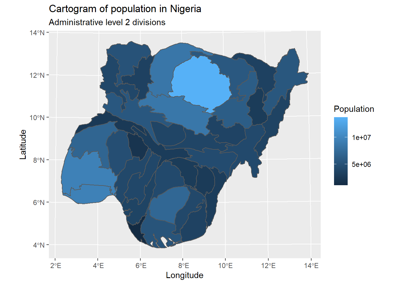

References

• wopr repository: https://github.com/wpgp/wopr
  
• ggplot2 package: https://ggplot2.tidyverse.org/
• Choropleth maps: https://www.data-to-viz.com/graph/choropleth.html
• Cartograms : https://www.data-to-viz.com/graph/cartogram.html

---

Last updated: 2023-01-07
Source code: https://github.com/rspatialdata/rspatialdata.github.io/blob/main/population.Rmd

Tutorial was complied using: (click to expand)

## R version 4.0.3 (2020-10-10)
## Platform: x86_64-w64-mingw32/x64 (64-bit)
## Running under: Windows 10 x64 (build 18363)
## 
## Matrix products: default
## 
## locale:
## [1] LC_COLLATE=English_United States.1252 
## [2] LC_CTYPE=English_United States.1252   
## [3] LC_MONETARY=English_United States.1252
## [4] LC_NUMERIC=C                          
## [5] LC_TIME=English_United States.1252    
## 
## attached base packages:
## [1] stats     graphics  grDevices utils     datasets  methods   base     
## 
## other attached packages:
##  [1] cartogram_0.2.2           wopr_0.4.6               
##  [3] ggmap_3.0.0               osmdata_0.1.5            
##  [5] malariaAtlas_1.0.1        ggthemes_4.2.4           
##  [7] here_1.0.1                MODIStsp_2.0.9           
##  [9] nasapower_4.0.7           terra_1.5-17             
## [11] rnaturalearthhires_0.2.0  rnaturalearth_0.1.0      
## [13] viridis_0.5.1             viridisLite_0.3.0        
## [15] raster_3.5-15             sp_1.4-5                 
## [17] sf_1.0-7                  elevatr_0.4.2            
## [19] kableExtra_1.3.4          rdhs_0.7.2               
## [21] DT_0.17                   forcats_0.5.1            
## [23] stringr_1.4.0             dplyr_1.0.4              
## [25] purrr_0.3.4               readr_2.1.2              
## [27] tidyr_1.1.4               tibble_3.1.6             
## [29] tidyverse_1.3.1           openair_2.9-1            
## [31] leaflet_2.1.1             ggplot2_3.3.5            
## [33] rgeoboundaries_0.0.0.9000
## 
## loaded via a namespace (and not attached):
##   [1] readxl_1.3.1        backports_1.4.1     systemfonts_1.0.4  
##   [4] plyr_1.8.7          selectr_0.4-2       splines_4.0.3      
##   [7] storr_1.2.5         crosstalk_1.2.0     urltools_1.7.3     
##  [10] digest_0.6.27       htmltools_0.5.2     fansi_0.4.2        
##  [13] magrittr_2.0.1      memoise_2.0.1       cluster_2.1.0      
##  [16] gdalUtilities_1.2.1 tzdb_0.3.0          modelr_0.1.8       
##  [19] vroom_1.5.7         xts_0.12.1          svglite_1.2.3.2    
##  [22] prettyunits_1.1.1   jpeg_0.1-9          colorspace_2.0-3   
##  [25] rvest_1.0.2         rappdirs_0.3.3      hoardr_0.5.2       
##  [28] haven_2.5.0         xfun_0.30           rgdal_1.5-23       
##  [31] crayon_1.5.1        jsonlite_1.8.0      hexbin_1.28.2      
##  [34] progressr_0.10.1    zoo_1.8-8           countrycode_1.2.0  
##  [37] glue_1.6.2          gtable_0.3.0        webshot_0.5.2      
##  [40] maps_3.4.0          scales_1.1.1        DBI_1.1.2          
##  [43] Rcpp_1.0.7          progress_1.2.2      units_0.8-0        
##  [46] bit_4.0.4           mapproj_1.2.8       htmlwidgets_1.5.4  
##  [49] httr_1.4.2          RColorBrewer_1.1-2  wk_0.5.0           
##  [52] ellipsis_0.3.2      pkgconfig_2.0.3     farver_2.1.0       
##  [55] sass_0.4.0          dbplyr_2.1.1        utf8_1.1.4         
##  [58] crul_1.2.0          tidyselect_1.1.0    labeling_0.4.2     
##  [61] rlang_1.0.2         munsell_0.5.0       cellranger_1.1.0   
##  [64] tools_4.0.3         cachem_1.0.6        cli_3.2.0          
##  [67] generics_0.1.2      broom_0.8.0         evaluate_0.15      
##  [70] fastmap_1.1.0       yaml_2.2.1          knitr_1.33         
##  [73] bit64_4.0.5         fs_1.5.2            s2_1.0.7           
##  [76] RgoogleMaps_1.4.5.3 nlme_3.1-149        xml2_1.3.2         
##  [79] compiler_4.0.3      rstudioapi_0.13     curl_4.3.2         
##  [82] png_0.1-7           e1071_1.7-4         reprex_2.0.1       
##  [85] bslib_0.3.1         stringi_1.5.3       highr_0.9          
##  [88] gdtools_0.2.4       lattice_0.20-41     Matrix_1.2-18      
##  [91] classInt_0.4-3      vctrs_0.3.8         slippymath_0.3.1   
##  [94] pillar_1.7.0        lifecycle_1.0.1     triebeard_0.3.0    
##  [97] jquerylib_0.1.4     data.table_1.14.2   bitops_1.0-7       
## [100] R6_2.5.0            latticeExtra_0.6-29 KernSmooth_2.23-17 
## [103] gridExtra_2.3       codetools_0.2-16    MASS_7.3-53        
## [106] assertthat_0.2.1    rjson_0.2.20        rprojroot_2.0.2    
## [109] withr_2.5.0         httpcode_0.3.0      mgcv_1.8-33        
## [112] parallel_4.0.3      hms_1.1.1           grid_4.0.3         
## [115] class_7.3-17        rmarkdown_2.11      packcircles_0.3.4  
## [118] lubridate_1.8.0

Corrections: If you see mistakes or want to suggest additions or modifications, please create an issue on the source repository or submit a pull request
Reuse: Text and figures are licensed under Creative Commons Attribution CC BY 4.0.